Search in book...
Toggle Font Controls
Create new playlist

Name your new playlist

Playlist description (optional)
Sign In

Email address

Password

Forgot Password?

or

Continue with Facebook

Continue with Google
Sign Up

Full Name

Email address

Confirm Email Address

Password

or

Continue with Facebook

Continue with Google

Chapter 10

Finite Element Modeling

Abstract

The finite element method (FEM) is used for modeling of physical systems in a wide variety of engineering disciplines, including structural dynamics, heat transfer, fluid dynamics, and aerodynamics. In this chapter, the application of FEM in modeling particle systems is introduced, which covers three aspects: (1) modeling of particle–particle interactions, (2) multiple particle finite element modeling (MPFEM), and (3) continuum modeling of powder compaction. A detailed discussion of the constitutive models used for powder compaction is presented, with particular reference to the Drucker–Prager-cap (DPC) model. In addition, methods for determination of material properties for finite element modeling with the DPC model are discussed in detail. Typical applications of FEM in modeling particle systems are illustrated.

Keywords

Contact modeling; Drucker–Prager-cap model; Finite discrete element method; Finite element modeling; Model calibration; Multiple particle finite element method; Particle interaction; Powder compaction

The finite element method (FEM) is one of the computational techniques for finding approximate solutions to differential and integral equations. Although FEM was developed in the first half of the twentieth century, with its initial application in solid mechanics, civil, and structural engineering, it has since advanced significantly into modeling of physical systems in a wide variety of engineering disciplines, including structural dynamics, heat transfer, fluid dynamics, and aerodynamics. In these and other fields of engineering and applied sciences, most real problems are complex in both geometry and boundary conditions. It is generally impossible to obtain analytical solutions for such problems, so approximate methods are needed. In FEM, a computational domain is generally set up within which the underlying physics can be defined using partial differential equations or integral equations. The defined computational domain is then subdivided into interconnecting simple geometric parts or subdomains, i.e., so-called finite elements, so that a set of element equations can be defined to approximate the original problem. An approximate solution for the whole domain can be obtained by solving these simple element equations. In outline, therefore, the practical application of FEM, i.e., finite element modeling, typically involves the following steps:

1. Defining a computational domain for the given problem.

2. Subdividing (i.e., discretizing) the computational domain into a set of elements, which is also referred to as mesh generation.

3. Developing integral or differential equations for a typical element (i.e., subdomain), and a set of algebraic equations (i.e., element equations) among the unknown parameters (degrees of freedom) of the elements.

4. Assembling a global system of algebraic equations from the element equations through transforming the local coordinates of the elements to the global coordinates (i.e., spatial transformation).

5. Applying essential boundary and initial conditions.

6. Solving the system of algebraic equations to obtain approximate values for the unknown parameters in the global coordinate system (i.e., using the global degrees of freedom).

7. Postprocessing to compute solutions and extract data of interest from the solutions obtained in Step 6.

A detailed discussion on the theory of FEM is outside the scope of this book; for this we refer readers to Zienkiewicz et al. (2013) and other FEM-related books. In this chapter, the application of FEM in modeling particle systems is introduced, which includes (1) modeling of particle–particle interactions; (2) multiple particle finite element modeling (MPFEM), and (3) continuum modeling, with an example in powder compaction.

10.1. Modeling of Particle–Particle Interaction

For the contact or impact between a particle and another particle or a wall, which are ubiquitous in particle technology, the boundary conditions at the contact are unknown a priori, as neither the actual contact surface nor the stresses and displacements on the contact surface are known prior to the solution of the problem. Contact/impact problems can also involve geometrical and material nonlinearity (i.e., complex material deformation behavior) so that it is very difficult if not impossible to obtain rigorous analytical solutions. However, with the advances in FEM, the contact/impact problems can now be effectively analyzed with desired accuracy. A detailed description of the principle of FEM for analyzing contact/impact problems can be found in Zienkiewicz et al. (1989), Hughes (1987), and Bathe (1982). Some distinct aspects involved in modeling of such problems using FEM are introduced in this section.

10.1.1. Contact Modeling Techniques

In FEM, contact boundaries are approximated by collections of polygons for three-dimensional (3D) problems and lines for two-dimensional (2D) applications. The polygons are normally either three-vertex triangular facets or four-vertex quadrilaterals. The polygons and lines composing the contact boundaries are referred to as contact segments. Each edge of the contact segment is known as a contact edge. A node on the contact edge or the contact segments is a contact node. A contact surface is then defined as the collection of all the contact segments that approximate to a complete physical boundary. Note that a contact object may have more than one contact surface.

In the contact between two different contact surfaces of either a single body or two contacting bodies, one of the contact surfaces is specified as a “slave” surface, and the other a “master” surface. The contact algorithms based on this specification are therefore known as master-slave algorithms (Zhong, 1993). Between two contact surfaces, the contact pressure results in an external load exerted on the contact body. In the FEM model, the contact load is replaced by a set of forces exerted at the nodes. Hence, the problem can be simplified by taking the nodal forces instead of the contact pressures as primary unknowns. The contact nodal forces can then be obtained by solving the governing equations for each contact segment (see, for example, Hughes et al., 1976 and Zhong, 1993), from which the contact pressure can in turn be calculated directly from the nodal forces.

The solution for the contact condition requires that the total number of the contacting slave nodes and the contact force at each be known a priori, implying that algorithms are needed to find the total number of contacting slave nodes and to determine the contact nodal force at each. The former is the task of contact searching procedures, while the latter requires certain contact constraint methods. Here contact search algorithms and the commonly used contact constraint methods (the kinematic constraint method and the penalty method) are introduced in Boxes 10.1 and 10.2, respectively.

Box 10.1 Contact Searching Procedure

In the master-slave method, the objective of the contact searching procedure is to determine the total number of contacting slave nodes n_c at time instant t and for each contacting slave node to find the corresponding contact point in the master segment. To determine n_c, a trial-and-error procedure is widely used. Assuming that the solution at time t − Δt is known, and that the total number of contacting slave nodes n_c and the position of a contact node in relation to all the contact segments are also known, it is possible to select new potential contact nodes at time t by evaluating the distance of a new potential contact node from any master segment/edge/node. It is then necessary to introduce a prescribed control distance, which can be specified either to be zero or on the basis of the relative velocities

{\dot{u}}_{c}

${\dot{u}}_{c}$

of the contact boundaries as

$l_{c} = Δ t {\dot{u}}_{c} (t - Δ t) \cdot N_{1} (t - Δ t)$ $l_{c} = Δ t {\dot{u}}_{c} (t - Δ t) \cdot N_{1} (t - Δ t)$

(10.1)

where N₁ is a unit normal vector at a potential target point. The selection of the potential contacting slave nodes is performed in three phases (Zhong, 1993): (1) a master node that is closest to the slave node being considered is found; (2) a master segment that contains the master node and is closest to the slave node is found as a target segment, and (3) the shortest distance between the slave node and its target master segment is calculated. If this distance is smaller than l_c, the slave node is then considered to be in contact with the master segment and regarded as a new potential contact slave node. Based on the selected potential contact slave nodes, an approximate solution is obtained. By enforcing the contact conditions at all the contact slave nodes, it may be found that the contact forces at some of the selected slave nodes are inconsistent with the physical conditions, implying that the mechanical contact condition is violated. A selected slave node that does not satisfy the mechanical contact condition is identified as an error node. To obtain a correct solution, all the error nodes must be removed from the selection of contacting nodes, and then the updated selection is obtained. The updated selection is used to find the solution. If no error nodes are found, the updated selection is regarded as the true selection, and the contact searching procedure can be terminated. For each identified slave node, the corresponding contact target point, defined as the closest point on the master segment to the slave node, can then be identified.

Box 10.2 Contact Constraint Methods: Kinematic versus Penalty

Once a potential contacting slave node and the corresponding target point on the master segment are found, contact constraints must be imposed to model the contact boundary conditions. Two approaches are commonly used to enforce the contact constraints: the kinematic constraint method and the penalty method.

In the kinematic constraint method, also known as the Lagrange multiplier method, constraints are enforced on the system of equations in the global coordinate system. With the FE discretization of the contact surface, impenetrability of contact (i.e., no node can penetrate its contacting surface) needs to be satisfied for all contact constraints, which can be established explicitly. With the kinematic constraint method, a Lagrange multiplier, having the contact forces as its elements, is introduced into the element equations. By treating the Lagrange multiplier vector as an unknown and solving the element equations using the given boundary conditions simultaneously, the Lagrange multiplier vector (i.e., the set of contact forces) can be determined.

The contact constraint condition is enforced exactly in the kinematic method. It should be noted that the enforcement of contact constraint is normally applied only on the slave nodes. Problems may hence arise when the master surface is discretized more finely than the slave surface, so that some master nodes may penetrate into the slave surface. Therefore, the master surface should be discretized with coarser elements than the slave surface.

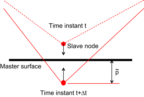
The penalty method uses an explicit approach to enforce the contact constraints. As illustrated in Fig. 10.1, a slave node is about to contact the master surface. At the time instant t, the slave node makes contact with the master surface and penetrates a distance

\tilde{p}

$\tilde{p}$

into the it. This is permitted so no action is taken to avoid the penetration at time t. However, at the next time instant t + Δt, an interface “spring” is added between the slave node and the master surface. The force generated from the interface spring is equal to the product of spring stiffness and the penetration distance

\tilde{p}

$\tilde{p}$

. The interface spring stiffness is normally determined as the multiplication of a penalty parameter

\tilde{α}

$\tilde{α}$

with the stiffness of the contacting bodies. Because the penalty method resolves any contact penetration that exists at the beginning of each increment and the contact force is directly computed by introducing the penalty parameters, it is therefore an explicit method.

In the penalty method, the contact constraints are enforced explicitly without any additional unknown, so the computation can be performed efficiently. Since the penetrations are controlled by the penalty parameters, the accuracy of the solution depends on the choice of these parameters. If the penalty parameters are too small, the resulted penetration may be too large, which may cause unacceptable calculation errors. If these parameters are too large, severe numerical problems may be caused and it may become impossible to obtain a solution. Thus the choice of the penalty parameters is critical.

Figure 10.1 Illustration of the penalty method.

10.1.2. Applications

As an example, consider the normal impact of a spherical particle with a planar surface as illustrated in Fig. 10.2. The sphere has a radius R = 10 μm and collides with the substrate at an incident velocity v_ni = 5.0 m/s. The sphere and the substrate are assumed to be elastic and have the same material properties: Young's modulus: 208.0 GPa; Poisson's ratio: 0.3; density: 7.85 × 10³ kg/m³. The normal impact shown in Fig. 10.2 is geometrically axisymmetric along the vertical axis passing through the center of the sphere; it can therefore be analyzed using a 2D FE model. Because of this symmetry, only half of the sphere and the substrate are considered (see Fig. 10.3).

The effects of impact are not confined to the contact area; a mechanical stress wave travels through both the particle and the substrate and carries energy away from the contact. The substrate in the FEM should be sufficiently large that the influence of the boundary constraints can be ignored. To choose the size of the substrate appropriately, it is necessary to estimate the maximum deformation by taking the loading condition and material properties into account. A systematic study on the effect of the substrate size (

L / R = 1 \sim 20

$L / R = 1 \sim 20$

) reported in Wu (2002) showed that a substrate of dimension L/R = 1 is too thin for modeling the impact accurately, even at low impact velocities. For impact with a substrate of dimension L/R ≥ 2, the effects of the boundary constraints and the propagation of the stress wave are sufficiently small, so that dimension L/R = 2 is adopted here.

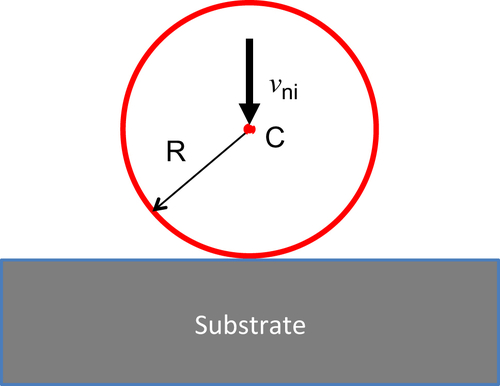
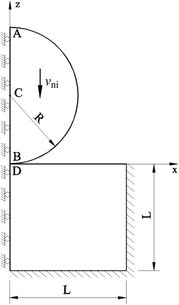
Figure 10.2 Illustration of the normal impact of a sphere with a planar surface.

Figure 10.3 The finite element model for the impact of a sphere with a substrate (Wu, 2002).

The corresponding FE model is shown in Fig. 10.4. Finer mesh is employed near the contact zone (Fig. 10.4(b)) in order to model the contact deformation more accurately, as the deformation is mainly localized to the region of the initial contact point (see Chapter 8).

The interaction between the sphere and the substrate is modeled with a master-slave slideline, consisting of two contact lines: one on the sphere side and the other on the substrate side. This type of slideline is based on the contact searching algorithm discussed in Box 10.1, and the kinematic constraint method (Box 10.2) is used to enforce the contact constraints. As specified in the kinematic constraint method, the master surface on the sphere side is discretized with coarse meshes, while finer mesh is used for the slave surface on the substrate side.

The collision process is modeled by specifying an initial velocity v_ni (i.e., 5.0 m/s) to every node inside the sphere. The boundary condition is illustrated in Fig. 10.3. Owing to the symmetry, all nodes along the z axis are constrained to move only in the z-direction (i.e., the displacement u_x = 0), while the nodes along the bottom line and the side edge of the substrate are fixed (i.e., u_x = μ_z = 0).

Figure 10.4 (a) Finite element model for the impact of a sphere with a half-space; (b) finer mesh used in the contact region (Wu, 2002).

Using the model presented in Fig. 10.4, and the given initial and boundary conditions, the response of each node in this model can then be solved using an FE solver. Here the solver DYNA2D (Whirley and Engelmann, 1992) is chosen but this type of problem can also be analyzed using other FE solvers, such as ABAQUS and ANSYS. From the response of each node, much information of interest can be obtained; some typical results are discussed in this section.

During the impact, both bodies deform and develop internal stresses. A typical pattern for the stress distribution at maximum compression is presented in Fig. 10.5, in which the effective stress is shown in Fig. 10.5(a), with the corresponding maximum shear stress in Fig. 10.5(b). It is clear that the pattern for the stresses inside the sphere is quite similar to that inside the substrate. The “+” signs in Fig. 10.5 indicate the location of the maximum value of the corresponding stresses. It can be seen that the maximum values of both the effective stress and shear stress are located inside the substrate at a depth of about half of the contact radius, implying that plastic deformation will initiate inside the substrate if the contacting bodies are elastic-plastic in nature.

From the FE analysis, the impact response, such as displacement and velocity at each node, the kinetic energy of each body and the contact force at the interface can also be obtained, as presented in Figs 10.6 and 10.7. Figure 10.6(a) shows the time evolutions of displacements at four distinct nodes: node A (the top); B (the bottom); C (the center), and D (the initial contact point of the substrate), as marked in Fig. 10.3. The corresponding velocity evolutions are given in Fig. 10.6(b). Figure 10.7(a) shows the evolution of the kinetic energy, and the evolution of the contact force is presented in Fig. 10.7(b). It can be seen that, for the whole impact process, there are two distinct phases: compression and restitution. The compression phase terminates when the nodal displacements and the contact force reach their maximum values, and the nodal velocities and the kinetic energy approach zero. Thereafter the restitution phase starts. The restitution phase ends when the nodal displacements and the contact force reduce to zero. After the separation of the two contacting bodies, the kinetic energy remains unchanged at a constant value close to the initial one, which implies that the energy loss due to stress wave propagation is negligible, and the coefficient of restitution is close to unity. The results shown in Fig. 10.6 also indicate that the deformation of the sphere is mainly concentrated in the bottom hemisphere as the nodal displacements at the top (A) and the center (C) of the sphere are essentially identical, while those at nodes C and B are very different.

Figure 10.5 Stress distributions inside the sphere and the substrate at the maximum compression: (a) the effective stress; (b) the maximum shear stress (Wu, 2002).

Figure 10.6 Time histories of (a) nodal displacements and (b) velocities during the impact of an elastic sphere with an elastic substrate. Nodes A, B, C, and D correspond to positions marked in Fig. 10.3 (Wu, 2002).

Figure 10.7 Time histories of (a) kinetic energy and (b) impact force during the impact of an elastic sphere with an elastic substrate (Wu, 2002).

From these impact responses, further information can be obtained, including the maximum pressure, the contact area (Fig. 8.4), the force–displacement relationship (see Figs 8.5 and 8.18), the duration of impact (Fig. 8.6), and the coefficient of restitution (Fig. 8.19), which provide physical insight into the contact/impact problems of particles.

Similar FE analysis can be readily applied to other more complex impact problems, including contact of irregularly shaped particles, interaction in the presence of surface energy (i.e., adhesive impacts), and interaction with liquid bridges, provided that an appropriate method can be established to model the liquid at the interface.

For modeling adhesive contact/impact using FEM, two techniques have been developed: (1) A body force model, in which adhesion is represented by intermolecular interactions, so that the van der Waals force between two bodies is modeled in the FE formulation as a body force derived from the Lennard-Jones potential (Zhang et al., 2011; Cho and Park, 2004; Sauser and Li, 2007; Sauer and Wriggers, 2009); (2) An interfacial adhesion model (Feng et al., 2009; Wang et al., 2012), in which the adhesive force is approximated by introducing spring elements. The deformation of the spring elements is modeled with a specified constitutive equation describing the relationship between the adhesion stress and the separation distance of the two surfaces.

Modeling particle interaction due to liquid bridges using FEM was attempted by Xu and Fan (2004), who applied the Laplace pressure and surface tension on the solids at the interface between the liquid and solid, and at the three-phase contact line respectively. The induced force and pressure were applied on the surfaces of the contacting bodies as the boundary conditions. In addition, the interaction between the liquid bridge and the deformation of the contacting bodies was considered. However, the liquid bridge was not modeled explicitly so its deformation during the contact was not considered, which deserves further investigation.

10.2. Multiple Particle Finite Element Modeling

In many applications, such as tableting and roll compaction, particle systems are subjected to high consolidation pressures, resulting in large deformations of particles. For these systems, the discrete element method (DEM) discussed in Chapter 9 is currently not applicable since large deformation (i.e., gross change of the geometry) of individual particles is not considered. For consolidation of particle systems, two computational approaches can be used:

1. Continuum modeling using FEM, in which a particle system is treated as a continuum instead of a collection of individual entities. This approach will be discussed in detail in Section 10.3;

2. MPFEM, which can be regarded as an extension of the approach described in Section 10.1 to model interactions of many particles simultaneously using FEM. This is sometimes referred to as the combined finite-discrete element method. In principle, it uses the FE procedure to model the deformation of a system consisting of discrete particles, each of which is considered explicitly.

In MPFEM, each particle is discretized with its own FEM mesh and its deformation individually modeled. As the particles interact with each other, their deformation depends on their loading conditions (including body forces, external forces, and contact forces) and the stress state. One of the key issues is then how to model the interaction between particles. The contact modeling techniques discussed in Section 10.1.1 can be used directly in MPFEM so that the contact can be modeled at each contact node. This approach was adopted by Procopio and Zavalinagos (2005), Zhang (2009), Frenning (2008, 2010), Harthong et al. (2009, 2012), Guner et al. (2015) and Gustafsson et al. (2013). It requires careful design of FE meshes so that the contact can be modeled accurately (generally requiring fine meshes) and with computational efficiency. An alternative approach was proposed by Ransing et al. (2000) and Lewis et al. (2005), who discretized the boundary of each particle with a layer of interface elements. The interface layer has a finite thickness Δ, a stiffness k, and a damping coefficient c. The contact force F is then calculated from the overlap δ and impact velocity v as follows

$F = \frac{k δ}{Δ - δ} + \frac{c v}{δ}$ $F = \frac{k δ}{Δ - δ} + \frac{c v}{δ}$

(10.2)

By introducing this interface layer, the kinematic behavior can be computed. Ransing et al. (2000) found that the choice of the stiffness and damping coefficient had negligible effect on the force–displacement relationship for the compression of particle systems, but could significantly affect the convergence stability and speed of the numerical calculation.

MPFEM is a useful approach as it combines the strength of conventional DEM, in which particles are modeled explicitly as individuals, and FEM, in which the deformation of individual particles and the interaction between them can be modeled. The combination can be used to model deformation of particles in a granular assembly under high compression pressures. It can also model large deformations of particles (see Fig. 10.8), arbitrary particle shapes (Fig. 10.9), and complex tooling geometries (Fig. 10.10). A further advantage is that the stress and strain distributions at the particle level can be determined. At the macroscopic level, both yield surfaces (Harthong et al., 2012) and overall compression behavior can be determined (Procopio and Zavalinagos, 2005; Frenning, 2008, 2010; Harthong et al., 2012).

However, MPFEM is very computationally intensive since each particle needs to be discretized into hundreds (even thousands) of elements, and the contact search needs to be carried out at the nodal level; this severely limits the number of particles that can be modeled. So far, the maximum number of particles in MPFEM analysis reported in literature is 1680 (Gustafsson et al., 2013), which is many orders of magnitude below the number of particles handled in powder handling and processing applications. Furthermore, using MPFEM, the FE mesh needs to be designed carefully so that both computational convergence and good accuracy can be obtained.

Figure 10.8 Modeling of compression of a mixture of ductile and brittle particles using FEM (Ransing et al., 2000).

Figure 10.9 Modeling of compression of arbitrarily shaped particles using FEM: distribution of shear stresses (Lewis et al., 2005).

Figure 10.10 Modeling of compression of deformable spheres in a complex shaped die using MPFEM: (a) model set up; (b) distribution of effective stresses (Guner et al., 2015).

10.3. Continuum Modeling of Powder Compaction

Powder compaction is a process used in the pharmaceutical, fine chemicals, powder metallurgy, ceramic, and agrochemical industries to manufacture particulate products, such as tablets, mechanical components, and pellets. During this process, powders are compressed in a mold (i.e., a die) under high pressure, and undergo a complicated response, ranging from particle rearrangement and particle deformation to fragmentation. Powder compaction can be adequately modeled using the DEM approach discussed in Chapter 9 if the applied pressure is very low so that the process is dominated by particle rearrangement and deformation of particles is negligible. Powder compaction involving high pressures and significant particle deformation can also be modeled using MPFEM, as discussed in Section 10.2, if only a limited number of particles or granules is involved. However, most powder compaction processes involve many millions of particles and high pressure so that significant particle deformation takes place. For these processes, neither DEM nor MPFEM is applicable.

A feasible alternative is the continuum approach using FEM, and it has been widely employed for modeling the compaction of metallic, ceramic, and pharmaceutical powders. Using this approach, powders are treated as continuous media instead of assemblies of individual particles, and the compaction processes are then described as boundary value problems, for which partial differential equations are developed to represent mass, energy, and momentum balances, and constitutive laws are introduced to describe stress-strain relationships and die-wall friction. The powders are generally modeled as elastic–plastic materials for which the yield behavior is approximated using appropriate yield models, widely known as the yield surfaces. (Here yield implies that the deformed material cannot recover to its initial state, such as after onset of plastic deformation.) The choice of material model and calibration of the associated material parameters are very important aspects in continuum modeling of powder compaction, which will be discussed in detail here.

10.3.1. Material Models

During powder compaction, a powder can be modeled as an elastic–plastic continuum and the deformation of the powder can be described using the incremental plasticity theory. In this approach, the total strain increment

ⅆ ε_{i j}

$ⅆ ε_{i j}$

can be decomposed into an elastic strain increment

ⅆ ε_{i j}^{e}

$ⅆ ε_{i j}^{e}$

and a plastic one

ⅆ ε_{i j}^{p}

$ⅆ ε_{i j}^{p}$

$ⅆ ε_{i j} = ⅆ ε_{i j}^{e} + ⅆ ε_{i j}^{p} (i = 1,3 and j = 1,3)$ $ⅆ ε_{i j} = ⅆ ε_{i j}^{e} + ⅆ ε_{i j}^{p} (i = 1,3 and j = 1,3)$

(10.3)

where subscript i and j indicate the coordinates.

The elastic behavior of isotropic materials (i.e., those for which the material properties are independent of direction) can be either linear or nonlinear. For elastic deformation, the relationship between macroscopic stress increment

ⅆ σ_{i j}

$ⅆ σ_{i j}$

and strain increment

ⅆ ε_{i j}^{e}

$ⅆ ε_{i j}^{e}$

can be given as (Timoshenko and Goodier, 1951):

$ⅆ ε_{i j}^{e} = \frac{ⅆ s_{i j}}{2 G} + \frac{ⅆ σ_{m}}{3 K} δ_{i j} (i = 1,3 and j = 1,3)$ $ⅆ ε_{i j}^{e} = \frac{ⅆ s_{i j}}{2 G} + \frac{ⅆ σ_{m}}{3 K} δ_{i j} (i = 1,3 and j = 1,3)$

(10.4)

where δ_ij is the Kronecker delta function (i.e., δ_ij = 1 if i = j, δ_ij = 0 if i ≠ j), σ_m is the mean stress and given as

$σ_{m} = \frac{1}{3} (σ_{11} + σ_{22} + σ_{33})$ $σ_{m} = \frac{1}{3} (σ_{11} + σ_{22} + σ_{33})$

(10.5)

s_ij is the deviatoric stress and given as

$s_{i j} = σ_{i j} - σ_{m} δ_{i j}$ $s_{i j} = σ_{i j} - σ_{m} δ_{i j}$

(10.6)

G and K are the shear and bulk moduli, respectively, which are material properties. For continuous solid materials, they are normally constants, but for powders, they are functions of the relative density. G and K are also related to the Young's modulus E and Poisson's ratio υ as follows

$E = \frac{9 G K}{3 K + G}$ $E = \frac{9 G K}{3 K + G}$

(10.7)

$υ = \frac{3 K - 2 G}{2 (3 K + G)}$ $υ = \frac{3 K - 2 G}{2 (3 K + G)}$

(10.8)

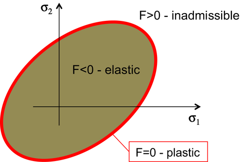
For elastic–plastic materials there is an elastic limit, above which plastic deformation initiates. This limit is defined by a yield criterion. For an unconfined uniaxial test, the yield criterion is simply that the yield stress Y is reached (see Fig. 8.2). However, when several stress components act on a material simultaneously, defining the yield criterion becomes complicated. Generally, the yield criterion is defined using a scalar yield function

$F [σ_{i j}, ς_{n}] = 0$ $F [σ_{i j}, ς_{n}] = 0$

(10.9)

where ς_n denotes n specific material parameters, such as the relative density. In the stress space, Eq. (10.9) defines a surface representing the elastic limit of the stress state, i.e., the set of maximal permissible stresses. In the plasticity theory, this surface is the so-called yield surface. An exemplar yield surface in 2D is illustrated in Fig. 10.11. The yield function is generally defined in such a way that the stress state is located inside the yield surface, i.e., F[σ_ij, ς_n] < 0, if the deformation is elastic; while the stress state is positioned on the yield surface, i.e., F[σ_ij, ς_n] = 0, if plastic deformation occurs. Note that it is inadmissible to have F[σ_ij, ς_n] > 0, i.e., it is impossible to have a stress state represented by a point outside the yield surface. This implies that in the plastic deformation range, the stress state can only be redistributed between different stress components so that the stress point is still on the yield surface but it may “slide” into a new position. The change from plastic deformation to elastic deformation (e.g., during unloading after powder compaction) leads to the stress point moving from the boundary of the yield surface to the inside, and vice versa.

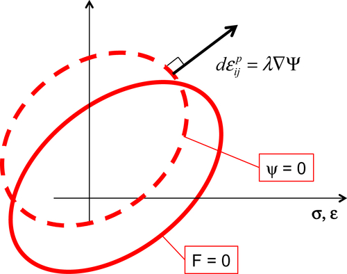
Figure 10.11 An example of yield surface in 2D.

Once plastic deformation takes place, the material may be subjected to further loading so that it may deform further. To describe the material response when plastic deformation prevails, a flow rule (or flow potential) needs to be defined to relate the plastic strain increment

ⅆ ε_{i j}^{p}

$ⅆ ε_{i j}^{p}$

at yield to the stress state. The plastic strain increment

ⅆ ε_{i j}^{p}

$ⅆ ε_{i j}^{p}$

can be given as (Green, 1972)

$ⅆ ε_{i j}^{p} = λ \frac{\partial Ψ}{\partial σ_{i j}} = λ \nabla Ψ$ $ⅆ ε_{i j}^{p} = λ \frac{\partial Ψ}{\partial σ_{i j}} = λ \nabla Ψ$

(10.10)

where λ is a plastic multiplier (i.e., a positive scalar of proportionality) and Ψ is the plastic flow potential, which is also a function of the stresses and material parameters, similarly to the yield function F[σ_ij, ς_n]. In the stress space, Ψ[σ_ij, ς_m] = 0 can also be represented as a surface, termed the flow potential surface. Because ∇Ψ is a vector normal to the surface described by Ψ[σ_ij, ς_m] = 0, Eq. (10.10) implies that the plastic strain increment

ⅆ ε_{i j}^{p}

$ⅆ ε_{i j}^{p}$

can be plotted as a vector normal to the surface with a length determined by the plastic multiplier λ, as illustrated in Fig. 10.12. The plastic flow potential Ψ needs to be defined for a given elastic–plastic material in a similar way to the yield function. For some materials, such as metals, the plastic flow potential can be approximated using exactly the same expression as the yield function, i.e., Ψ[σ_ij, ς_m] = F[σ_ij, ς_m]. In this case, Eq. (10.10) becomes

$ⅆ ε_{i j}^{p} = λ \frac{\partial F}{\partial σ_{i j}} = λ \nabla F$ $ⅆ ε_{i j}^{p} = λ \frac{\partial F}{\partial σ_{i j}} = λ \nabla F$

(10.11)

Figure 10.12 Illustration of the plastic strain increment in 2D.

Since the flow rule is associated with the yield function (Eq. (10.11)), this is so-called associated flow. If Ψ[σ_ij, ς_m] has a different expression from F[σ_ij, ς_m], the flow rule is nonassociated, because the plastic strain increment is not associated with the yield function. The nonassociated flow rule can be applied to most elastic–plastic materials.

Various yield surfaces were proposed to describe the plastic behavior of particulate materials, including the Drucker–Prager–Cap (DPC) model (Drucker and Prager, 1952), the Cam-Clay model (Schofield and Wroth 1968), and the Gurson model (Dimaggio and Sandler, 1971). Originally developed for soil mechanics, these have been used for analyzing consolidation of soils, the compaction of metallic, ceramic, and pharmaceutical powders (Aydin et al., 1996; Wu et al., 2005; Coube and Riedel, 2000; Sinka et al., 2003; Michrafy et al., 2002). Among these models, the DPC model is the most widely used yield surface for modeling powder compaction, because it can describe both the shear failure and the plastic yield of particulate materials; in addition, it can be readily calibrated experimentally for most powders. It is therefore discussed in the next section.

10.3.2. DPC Model

The DPC model was initially developed as an extension of the Mohr–Coulomb model (see Chapter 7) with a compaction surface introduced as the yield criterion, so it originally consisted of a shear failure segment F_s that is essentially the Mohr–Coulomb failure line and a cap segment F_c (Dracker and Prager, 1952). In order to ensure computational stability, a modified DPC model was developed and implemented in some FE solvers, such as ABAQUS, in which a transition segment F_t was introduced to provide a smooth surface bridging the shear failure segment and the cap segment (ABAQUS, 2013). These three segments are generally defined using two stress invariants: the hydrostatic pressure p and the von Mises equivalent stress q in the (p, q) plane (see Fig. 10.13),

$p = \frac{1}{3} (σ_{1} + σ_{2} + σ_{3})$ $p = \frac{1}{3} (σ_{1} + σ_{2} + σ_{3})$

(10.12)

$q = \sqrt{\frac{1}{6} [{(σ_{1} - σ_{2})}^{2} + {(σ_{2} - σ_{3})}^{2} + {(σ_{3} - σ_{1})}^{2}]}$ $q = \sqrt{\frac{1}{6} [{(σ_{1} - σ_{2})}^{2} + {(σ_{2} - σ_{3})}^{2} + {(σ_{3} - σ_{1})}^{2}]}$

(10.13)

where σ_i (i = 1, 2, 3) are the principal stresses.

The shear failure surface F_s is a straight line determined by the cohesion d and the angle of friction β:

$F_{s} [p, q] = q - p \tan β - d = 0$ $F_{s} [p, q] = q - p \tan β - d = 0$

(10.14)

This defines a criterion for the occurrence of shear flow. For a given material, if the stress state defined by the hydrostatic pressure p and the von Mises equivalent stress q satisfies Eq. (10.14), i.e., F_s[p, q] = 0, shear failure is induced.

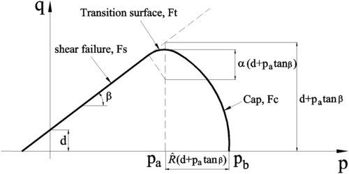
Figure 10.13 The Drucker–Prager–Cap model (Wu et al., 2005).

The cap surface F_c describes compaction and hardening of a material. If the stress state positions on the cap surface, densification and hardening occurs. The cap surface is an elliptical curve of constant eccentricity in the p–q plane and intersects the hydrostatic pressure axis (i.e., p axis). It is defined by:

$F_{c} [p, q] = \sqrt{{(p - p_{a})}^{2} + {(\frac{\hat{R} q}{1 + α - α / \cos β})}^{2}} - \hat{R} (d + p_{a} \tan β) = 0$ $F_{c} [p, q] = \sqrt{{(p - p_{a})}^{2} + {(\frac{\hat{R} q}{1 + α - α / \cos β})}^{2}} - \hat{R} (d + p_{a} \tan β) = 0$

(10.15)

where

\hat{R}

$\hat{R}$

and α are parameters defining the shape of the cap surface and the transition surface, respectively. p_a is an evolution parameter characterizing the hardening or softening behavior driven by the volumetric plastic strain,

ε_{v}^{p}

$ε_{v}^{p}$

, and given as:

$p_{a} = \frac{p_{b} - \hat{R} d}{1 + \hat{R} \tan β}$ $p_{a} = \frac{p_{b} - \hat{R} d}{1 + \hat{R} \tan β}$

(10.16)

where p_b is the hydrostatic pressure that defines the position of the cap. p_b is generally defined as a function of the volumetric plastic strain

ε_{v}^{p}

$ε_{v}^{p}$

, i.e.,

$p_{b} = f [ε_{v}^{p}]$ $p_{b} = f [ε_{v}^{p}]$

(10.17)

Equation (10.17) determines hardening or softening of the cap surface: hardening is caused by volumetric plastic compaction, while softening is induced by volumetric plastic dilation.

The transition surface is always relatively small and controlled by the parameter α with a typical value of 0.01-0.05. The transition surface is given by:

$F_{t} [p, q] = \sqrt{{(p - p_{a})}^{2} + {[q - (1 - \frac{α}{\cos β}) (d + p_{a} \tan β)]}^{2}} - α (d + p_{a} \tan β) = 0$ $F_{t} [p, q] = \sqrt{{(p - p_{a})}^{2} + {[q - (1 - \frac{α}{\cos β}) (d + p_{a} \tan β)]}^{2}} - α (d + p_{a} \tan β) = 0$

(10.18)

Two flow potentials are defined as the plastic flow rules: an associated flow potential Ψ_c on the cap surface and a nonassociated flow potential Ψ_s for the shear failure surface and the transition surface. The associated flow potential Ψ_c and the nonassociated flow potential Ψ_s are defined as

$Ψ_{c} [p, q] = \sqrt{{(p - p_{a})}^{2} + {(\frac{\hat{R} q}{1 + α - α / \cos β})}^{2}}$ $Ψ_{c} [p, q] = \sqrt{{(p - p_{a})}^{2} + {(\frac{\hat{R} q}{1 + α - α / \cos β})}^{2}}$

(10.19)

$Ψ_{s} [p, q] = \sqrt{{[(p - p_{a}) \tan β]}^{2} + {(\frac{q}{1 + α - α / \cos β})}^{2}}$ $Ψ_{s} [p, q] = \sqrt{{[(p - p_{a}) \tan β]}^{2} + {(\frac{q}{1 + α - α / \cos β})}^{2}}$

(10.20)

In the (p, q) plane, Eqs (10.19) and (10.20) represent two elliptic segments of a continuous and smooth potential surface, as shown in Fig. 10.14.

The DPC model introduces six parameters: d, β,

\hat{R}

$\hat{R}$

, p_a, α, and p_b. They are not necessarily constant for powders but it was shown that d, β,

\hat{R}

$\hat{R}$

, p_a are functions of the relative density, and p_b varies with the volumetric plastic strain (Eq. (10.17)). The cohesion d and internal frictional angle β define the shear failure surface;

\hat{R}

$\hat{R}$

and p_a determine the cap surface; α is one of the parameters defining the transition surface; and p_b specifies the hardening or softening of the cap surface. All six parameters are required to define the constitutive model for a given powder, in addition to the elasticity parameters, such as Young's modulus E and Poisson's ratio υ.

10.3.3. Determination of Constitutive Properties

In order to use the models discussed above, all parameters have to be determined from experimental measurements on the material under consideration. This exercise is called experimental calibration of the constitutive models (or simply “model calibration”). Full calibration of the models requires triaxial compression test data. In the triaxial test, the stresses acting on a test sample can be controlled separately in three directions so that a wide range of stress states can be achieved, and stress probing can also be performed to identify the yield, loading, hardening, and softening at different stress levels. However, the triaxial test requires a sophisticated testing system and complicated data analysis, and its application is limited to scientific research. Furthermore, powders can deform significantly during triaxial testing, which makes the interpretation of the test data extremely difficult.

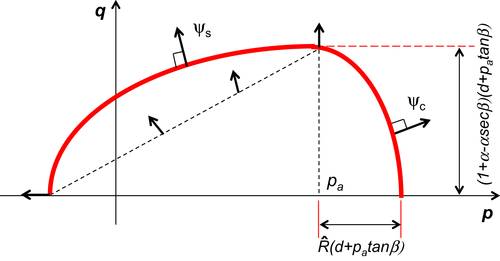
Figure 10.14 Illustration of the plastic flow rules in the Drucker–Prager–Cap model (Aydin et al., 1996).

Alternatively, model calibration using simple and standard test systems has also been developed, which generally involves uniaxial compression in a die instrumented with radial pressure sensors; in addition to measuring the radial stresses, diametrical compression and unconfined uniaxial compression can also be measured, as illustrated in Fig. 10.15.

10.3.3.1. Young’s modulus E and Poisson’s ratio υ

Determination of elastic properties (i.e., Young's modulus E and Poisson's ratio υ) can be achieved using the uniaxial compression test with an instrumented cylindrical die (Aydin et al., 1996; Wu et al., 2005; Michrafy et al., 2002). During the test, a powder is first compressed to a specified maximum compression force and then unloaded. The typical relationship between the axial stress σ_z and axial strain ε_z (i.e., the stress and strain in the z-direction) is illustrated in Fig. 10.16. During loading, the stress increases with the strain at an increasing rate. In the early stage of unloading, the stress decreases linearly with the strain, implying that elastic deformation dominates.

For uniaxial compression:

$σ_{1} = σ_{z}$ $σ_{1} = σ_{z}$

(10.21)

$σ_{2} = σ_{3} = σ_{r}$ $σ_{2} = σ_{3} = σ_{r}$

(10.22)

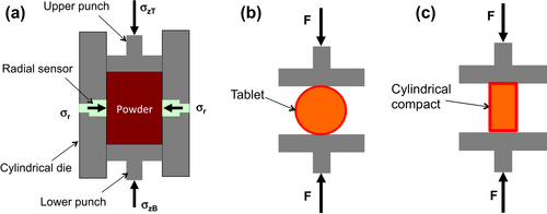
Figure 10.15 Some tests involved in model calibration: (a) uniaxial compression, (b) diametrical compression, and (c) unconfined uniaxial compression.

Figure 10.16 The variation of axial stress with axial strain during compaction (Wu et al., 2005).

Using Eqs (10.12) and (10.13), we have

$p = \frac{1}{3} (σ_{z} + 2 σ_{r})$ $p = \frac{1}{3} (σ_{z} + 2 σ_{r})$

(10.23)

$q = \frac{1}{\sqrt{3}} | σ_{z} - σ_{r} |$ $q = \frac{1}{\sqrt{3}} | σ_{z} - σ_{r} |$

(10.24)

From the measurement of the radial stress, the evolution of stress states (p, q) during the whole compaction process can be obtained. Figure 10.17 shows the corresponding evolution of stress states in the p–q plane. During loading, the stress increases from (0, 0) (point A, in Fig. 10.17) until the maximum compression is reached (point B), at which point the powder has been plastically deformed (i.e., irreversible deformation has taken place). Therefore, from the incremental plasticity theory, point B should be on the yield surface or, in other words, it should be positioned on the cap surface in the DPC model.

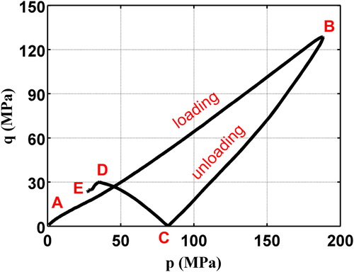
Figure 10.17 The variation of deviatoric stress with mean stress during compaction (Wu et al., 2005).

During unloading, elastic deformation takes place and the stress state moves away from the yield surface. As the axial stress σ_z decreases, at a certain point it will have the same value as the radial stress σ_r, i.e., σ_z = σ_r. From Eq. (10.24), q = 0. This is the hydrostatic state, denoted as point C in Figs 10.16 and 10.17. Once the unloading progresses beyond the hydrostatic state, the axial stress becomes smaller than the radial stress (i.e., σ_z < σ_r). Since the von Mises equivalent stress q is nonnegative, as shown in Eq. (10.24), q increases as the unloading continues, until it reaches the shear failure surface F_s [p, q] = 0 (point D). The magnitudes of the slopes of BC and CD in the (p, q) plane are very close, provided that the change in relative density of the powder system is not significant. Further unloading will be accompanied by dilation (DE).

For elastic unloading from uniaxial compaction in a cylindrical die,

$ⅆ ε_{11} = ⅆ ε_{z}$ $ⅆ ε_{11} = ⅆ ε_{z}$

(10.25a)

$ⅆ ε_{22} = ⅆ ε_{r} = 0$ $ⅆ ε_{22} = ⅆ ε_{r} = 0$

(10.25b)

$ⅆ ε_{33} = ⅆ ε_{θ} = 0$ $ⅆ ε_{33} = ⅆ ε_{θ} = 0$

(10.25c)

Substituting Eqs (10.21)–(10.25) into Eq. (10.4), we obtain

$\frac{ⅆ σ_{z}}{ⅆ ε_{z}} = K + \frac{4}{3} G$ $\frac{ⅆ σ_{z}}{ⅆ ε_{z}} = K + \frac{4}{3} G$

(10.26a)

$\frac{ⅆ q}{ⅆ p} = \frac{2 G}{\sqrt{3} K}$ $\frac{ⅆ q}{ⅆ p} = \frac{2 G}{\sqrt{3} K}$

(10.26b)

Equation (10.26) indicates that the slope of the unloading curve (BC or CD) in Fig. 10.16 can be described using Eq. (10.26a), while the slopes of BC and CD in Fig. 10.17 can be approximated using Eq. (10.26b). Therefore, we have

$K + \frac{4}{3} G = \frac{σ_{z B} - σ_{z C}}{ε_{z B} - ε_{z C}}$ $K + \frac{4}{3} G = \frac{σ_{z B} - σ_{z C}}{ε_{z B} - ε_{z C}}$

(10.27a)

$\frac{2 G}{\sqrt{3} K} = \frac{q_{B} - q_{C}}{p_{B} - p_{C}} = \frac{q_{B}}{p_{B} - p_{C}}$ $\frac{2 G}{\sqrt{3} K} = \frac{q_{B} - q_{C}}{p_{B} - p_{C}} = \frac{q_{B}}{p_{B} - p_{C}}$

(10.27b)

where the subscripts B and C denote the values at points B and C in Figs 10.16 and 10.17, respectively.

From Eq. (10.27), the bulk modulus K and shear modulus G can be calculated. Consequently, the Young's modulus E and Poisson's ratio υ can be determined using Eqs (10.7) and (10.8). It should be noted that the Young's modulus E and Poisson's ratio υ obtained using Eq. (10.27) are for the powder with a specific relative density, which was achieved with a maximum compression pressure of σ_zB, and therefore assumes that dilation during unloading is insignificant. To obtain Young's modulus E and Poisson's ratio υ at different relative densities, the powder needs to be compressed at appropriate maximum pressures, i.e., σ_zB, and for each compression, one set of values for Young's modulus E and Poisson's ratio υ can be determined. As a result, the variation of E and υ with relative density can be determined. The use of Eq. (10.27) to obtain the elastic properties for powders undergoing significant dilation during unloading needs caution, as the variation in the relative density during unloading can be very large and thus significant errors may be introduced. For powders undergoing significant dilation during unloading, Eq. (10.26) can be used to determine the E and υ at different stress states during unloading, and the relative density can also be calculated from the increment axial strain so that the relationship between the elastic properties (E and υ) and the relative density can be determined.

10.3.3.2. Cohesion d and angle of friction β

The cohesion d and the angle of friction β can be determined from either (1) uniaxial compression in an instrumented die or (2) a combination of diametrical compression and unconfined uniaxial compression tests.

From uniaxial compression in an instrumented die, the nonlinear part of the stress–strain curve at the very end of unloading (DE in Fig. 10.16) is attributed to shear failure, and in the p–q plane, the corresponding stress state falls on the shear failure surface. Therefore, by fitting the regime DE with a straight line in the p–q plane (see Fig. 10.17), the cohesion d and the friction angle β can be determined as follows

$d = \frac{p_{E} q_{D} - p_{D} q_{E}}{p_{E} - p_{D}}$ $d = \frac{p_{E} q_{D} - p_{D} q_{E}}{p_{E} - p_{D}}$

(10.28a)

$β = \tan^{- 1} (\frac{q_{D} - q_{E}}{p_{D} - p_{E}})$ $β = \tan^{- 1} (\frac{q_{D} - q_{E}}{p_{D} - p_{E}})$

(10.28b)

This approach only involves the uniaxial compression test and can only be used for powders with insignificant dilation during unloading. In practice, some degree of dilation will inevitably occur, which will introduce a degree of error. A further practical problem in these measurements is that the stress level during unloading is very small by comparison with the maximum compression level, and so cannot be determined with high accuracy.

Alternatively, a combination of diametrical compression (Fig. 10.15(b)) and unconfined uniaxial compression tests (Fig. 10.15(c)) can be performed to determine the cohesion d and the angle of friction β. For these tests, it is critical to prepare some compacts with the same relative densities so that two different tests can be performed with samples of the same relative density. The maximum tensile stress σ_t in the diametrical compression test (Fig. 10.15(b)) can be calculated from the maximum break force using Eq. (2.36), while the maximum compression stress σ_c in the unconfined uniaxial compression test (Fig. 10.15(c)) can be determined from the break force F and the cross-sectional area of the cylindrical compact, i.e.,

$σ_{c} = \frac{4 F}{π D^{2}}$ $σ_{c} = \frac{4 F}{π D^{2}}$

(10.29)

where D is the diameter of the compact. When the compact breaks during diametrical compression, the stress state at the center can be given as (Cunningham et al., 2004)

$σ_{1} = σ_{t}$ $σ_{1} = σ_{t}$

(10.30a)

$σ_{2} = - 3 σ_{t}$ $σ_{2} = - 3 σ_{t}$

(10.30b)

$σ_{3} = 0$ $σ_{3} = 0$

(10.30c)

Using Eqs (10.12) and (10.13), we have

$p = \frac{2}{3} σ_{t}$ $p = \frac{2}{3} σ_{t}$

(10.31a)

$q = \sqrt{13} σ_{t}$ $q = \sqrt{13} σ_{t}$

(10.31b)

Similarly, for the unconfined uniaxial compression test, we have

$σ_{1} = - σ_{c}$ $σ_{1} = - σ_{c}$

(10.32a)

$σ_{2} = σ_{3} = 0$ $σ_{2} = σ_{3} = 0$

(10.32b)

and

$p = \frac{1}{3} σ_{c}$ $p = \frac{1}{3} σ_{c}$

(10.33a)

$q = σ_{c}$ $q = σ_{c}$

(10.33b)

Substituting Eqs (10.31) and (10.33) into (10.14), and solving the system of equations, we obtain

$d = \frac{(\sqrt{13} - 2) σ_{t} σ_{c}}{σ_{c} - 2 σ_{t}} = \frac{2.33 σ_{t} σ_{c}}{σ_{c} - 2 σ_{t}}$ $d = \frac{(\sqrt{13} - 2) σ_{t} σ_{c}}{σ_{c} - 2 σ_{t}} = \frac{2.33 σ_{t} σ_{c}}{σ_{c} - 2 σ_{t}}$

(10.34a)

$β = \tan^{- 1} [3 (\frac{σ_{c} - d}{σ_{c}})]$ $β = \tan^{- 1} [3 (\frac{σ_{c} - d}{σ_{c}})]$

(10.34b)

Once the strength of a powder compact in diametrical compression and unconfined uniaxial compression is known (i.e., σ_t and σ_c), the cohesion d and the angle of friction β can be calculated using Eq. (10.34). This is a very robust approach for determining the cohesion d and the angle of friction β when the relative density is high, i.e., when strong compacts can be produced for testing. It may become problematic for compacts of low relative densities, as they tend to be too fragile to be used in these tests.

The two approaches introduced above are complementary so that they could be used in combination for determining the cohesion d and the angle of friction β over a wide range of relative densities. The first approach can be used for powders at low relative densities (i.e., under low compression pressure in uniaxial compression), for which the dilation during unloading is generally very small so that the measurement error can be minimized, while the second approach can be used for powder compacts with high relative densities as they are generally strong enough to be tested under diametrical compression and unconfined uniaxial compression.

10.3.3.3. Cap parameters: $\hat{R}$ $\hat{R}$ , p_a, α, and p_b

Four additional parameters,

\hat{R}

$\hat{R}$

, p_a, α, and p_b are required to define the cap surface and the transition surface. Among these parameters, α is generally very small with a value of 0.01–0.05. Within this range, the variation of α has little effect on the yield behavior, as it is introduced primarily to ensure computational stability. It may therefore be chosen arbitrarily within this range.

The values of

\hat{R}

$\hat{R}$

and p_a can be determined from the analysis of the stress state on the cap surface. As discussed above, point B in Fig. 10.17 is located on the cap surface. Hence from Eq. (10.15), we have

$F_{c} [p_{B}, q_{B}] = \sqrt{{(p_{B} - p_{a})}^{2} + {(\frac{\hat{R} q_{B}}{1 + α - α / \cos β})}^{2}} - \hat{R} (d + p_{a} \tan β) = 0$ $F_{c} [p_{B}, q_{B}] = \sqrt{{(p_{B} - p_{a})}^{2} + {(\frac{\hat{R} q_{B}}{1 + α - α / \cos β})}^{2}} - \hat{R} (d + p_{a} \tan β) = 0$

(10.35)

At point B, the plastic strain increment in the radial direction

ⅆ ε_{r}^{p}

$ⅆ ε_{r}^{p}$

can be assumed to be zero, as the deformation of the powder in the radial direction is constrained by the die wall. Thus, using Eq. (10.10), the radial plastic strain increment can be given as

$ⅆ ε_{r}^{p} = λ \frac{\partial Ψ_{c} (p_{B}, q_{B})}{\partial σ_{r}} = 0$ $ⅆ ε_{r}^{p} = λ \frac{\partial Ψ_{c} (p_{B}, q_{B})}{\partial σ_{r}} = 0$

(10.36)

Since λ is a positive scalar, to satisfy Eq. (10.36), we have

${\frac{\partial Ψ_{c}}{\partial σ_{r}} |}_{(p_{B}, q_{B})} = 0$ ${\frac{\partial Ψ_{c}}{\partial σ_{r}} |}_{(p_{B}, q_{B})} = 0$

(10.37)

Substituting Eq. (10.19) into Eq. (10.37) gives

${2 (p - p_{a}) \frac{\partial p}{\partial σ_{r}} |}_{(p_{B}, q_{B})} + \frac{2 {\hat{R}}^{2} q}{{(1 + α - α / \cos β)}^{2}} {\frac{\partial q}{\partial σ_{r}} |}_{(p_{B}, q_{B})} = 0$ ${2 (p - p_{a}) \frac{\partial p}{\partial σ_{r}} |}_{(p_{B}, q_{B})} + \frac{2 {\hat{R}}^{2} q}{{(1 + α - α / \cos β)}^{2}} {\frac{\partial q}{\partial σ_{r}} |}_{(p_{B}, q_{B})} = 0$

(10.38)

Using Eqs (10.23), (10.24), and (10.38), we obtain

$- \frac{2}{3} (p_{B} - p_{a}) + \frac{{\hat{R}}^{2} q_{B}}{{(1 + α - α / \cos β)}^{2}} = 0$ $- \frac{2}{3} (p_{B} - p_{a}) + \frac{{\hat{R}}^{2} q_{B}}{{(1 + α - α / \cos β)}^{2}} = 0$

(10.39)

Hence, the cap parameter

\hat{R}

$\hat{R}$

can be solved from Eq. (10.39) as

$\hat{R} = \sqrt{\frac{2 {\hat{α}}^{2} (p_{B} - p_{a})}{3 q_{B}}}$ $\hat{R} = \sqrt{\frac{2 {\hat{α}}^{2} (p_{B} - p_{a})}{3 q_{B}}}$

(10.40)

where

\hat{α} = 1 + α - α / \cos β

$\hat{α} = 1 + α - α / \cos β$

Substituting Eq. (10.40) into Eq. (10.39), p_a can then be solved in terms of the known parameters p_B, q_B, α, d, and β and is given as (Han et al., 2008)

$p_{a} = \frac{- 3 q_{B} - 4 d {\hat{α}}^{2} \tan β + \sqrt{9 q_{B}^{2} + 24 d q_{B} {\hat{α}}^{2} \tan β + 8 {\hat{α}}^{2} (3 p_{B} q_{B} + 2 q_{B}^{2}) \tan^{2} β}}{4 {\hat{α}}^{2} \tan^{2} β}$ $p_{a} = \frac{- 3 q_{B} - 4 d {\hat{α}}^{2} \tan β + \sqrt{9 q_{B}^{2} + 24 d q_{B} {\hat{α}}^{2} \tan β + 8 {\hat{α}}^{2} (3 p_{B} q_{B} + 2 q_{B}^{2}) \tan^{2} β}}{4 {\hat{α}}^{2} \tan^{2} β}$

(10.41)

Once p_a is determined, the cap parameter

\hat{R}

$\hat{R}$

can be calculated from Eq. (10.40). Hence, using Eq. (10.16), p_b can be determined, i.e.,

$p_{b} = \hat{R} d + p_{a} (1 + \hat{R} \tan β)$ $p_{b} = \hat{R} d + p_{a} (1 + \hat{R} \tan β)$

(10.42)

The corresponding volumetric plastic strain can be calculated from the relative densities at point B (i.e., the relative density at the maximum compression), ρ_B, and at point A, ρ_A (i.e., the initial relative density prior to compaction) as follows

$ε_{v}^{p} = ε_{v B}^{p} = \ln (\frac{ρ_{B}}{ρ_{A}})$ $ε_{v}^{p} = ε_{v B}^{p} = \ln (\frac{ρ_{B}}{ρ_{A}})$

(10.43)

Strictly speaking, the measured cap parameters

\hat{R}

$\hat{R}$

, p_a, and p_b are related to the material state at maximum compression (i.e., point B in Figs 10.16 and 10.17); hence, the corresponding relative density and volumetric plastic strain should be ρ_B and

ε_{v B}^{p}

$ε_{v B}^{p}$

, respectively. To obtain the dependence of these parameters on relative density, the powder needs to be compressed to different maximum pressures. For each compaction, a specific value for each of these parameters can be obtained, together with the corresponding volumetric plastic strain

ε_{v}^{p}

$ε_{v}^{p}$

. Hence the cap parameters

\hat{R}

$\hat{R}$

and p_a can be obtained as functions of relative density, as can p_b as a function of the volumetric plastic strain

ε_{v}^{p}

$ε_{v}^{p}$

. For some applications, a density-independent calibration can be performed, which is discussed in Box 10.3.

Box 10.3 Density-Independent Calibration

If the effect of relative density on the constitutive parameters is insignificant, i.e., the elastic properties (Young's modulus and Poisson's ratio), the cohesion d, the angle of friction β, and the cap parameters

\hat{R}

$\hat{R}$

and p_a are independent of the relative density, the relationship between p_b and

ε_{v}^{p}

$ε_{v}^{p}$

may also be determined from a single set of compaction data, as adopted by Aydin et al. (1996), Michrafy et al. (2002), and Wu et al. (2005). In this case, the Young's modulus and Poisson's ratio are constants, and the unloading curves in the stress-strain diagram will be parallel to each other if the powder is compressed to various maximum compression pressures, as the slopes of the unloading curves are identical as defined by Eq. (10.26a). The volumetric plastic strain can be determined as:

$ε_{v}^{p} = ε_{z} - \frac{σ_{z}}{K + 4 G / 3}$ $ε_{v}^{p} = ε_{z} - \frac{σ_{z}}{K + 4 G / 3}$

(10.44)

Using the corresponding stress state (p, q) on the loading curve, p_a can be determined from Eq. (10.41) by replacing (p_B, q_B) with (p, q), and p_b can then be determined using Eq. (10.42). Therefore, the variation of p_b with

ε_{v}^{p}

$ε_{v}^{p}$

can be determined.

10.3.3.4. DPC model calibration procedure

The calibration procedure for the DPC model using uniaxial compression and diametrical compression described above can be summarized as follows:

Step 1:

Produce cylindrical samples of a certain relative density D₁ and perform diametrical compression and unconfined uniaxial compression tests to obtain the tensile stress σ_t and the compression strength σ_c, respectively. Use Eq. (10.34) to calculate the cohesion d₁ and the internal frictional angle β₁.

Step 2:

Perform uniaxial compression (loading and unloading) of the sample powder in an instrumented die to a maximum compression pressure that results in a relative density of the same value as D₁ at the maximum compression. Plot σ_z versus ε_z, and p versus q from the uniaxial data in the similar way to that shown in Figs 10.16 and 10.17. Identify the critical stress states pointed out as A, B, C, D, and E. Use Eq. (10.27) to calculate the bulk modulus K₁ and shear modulus G_1, then calculate the Young's modulus E₁ and Poisson's ratio υ₁ using Eqs (10.7) and (10.8).

Step 3:

If it is impossible to get the cohesion d₁ and the internal frictional angle β₁ in Step 1, especially for powders in a certain relative density range, fit the regime DE in the p–q plot using a straight line, and calculate the cohesion d₁ and the internal frictional angle β₁ using Eq. (10.28).

Step 4:

Choose a value for α ( = 0.01∼0.05), calculate

\hat{R}

$\hat{R}$

using Eq. (10.40), p_a from Eq. (10.41) and p_b and

ε_{v}^{p}

$ε_{v}^{p}$

from Eqs (10.42) and (10.43).

Repeating the above steps for different relative densities, the variations of the DPC parameters with relative densities can then be obtained. Tables 10.1–10.6 list a collection of DPC-based constitutive parameters for various powders reported in the literature.

10.3.4. Modeling Procedure and Applications

The theoretical approaches discussed in this chapter together with other algorithms can be implemented in a computer program, which forms the FEM solver. A variety of FE packages are available as FEM solvers. Using these solvers to model the compaction of a powder, a range of input parameters are needed, which can be classified into two categories: material parameters and process parameters. For a given powder, as illustrated in Fig. 10.18, it is necessary not only to choose a material model that can represent the deformation behavior of the powder, but also to perform model calibration (see Section 10.3.3) so that the input material parameters are specific to the powder considered. Process parameters are also needed so that the geometry and process conditions can be specified; these are generally defined in the FE model as boundary and loading conditions. Using these input parameters, FE modeling can be performed to explore the responses of the system, which include the response of the powder during the process, e.g., compaction behavior, properties of final products, such as density and stress distributions, and the response of the tooling if it is of interest. In this section, typical output from FE modeling will be discussed in order to illustrate the FE capability.

Table 10.1

Density-Independent DPC Parameters Reported in the Literature

Powder	E (GPa)	v	d (MPa)	β(^o)	α		p_b (MPa)
α-Al₂O₃ (AKP-30), an agglomerated alumina powder (Aydin et al., 1996)	9.03	0.28	5.50	16.50	0.03	0.56	$p_{b} = c_{1} + c_{2} \times 10^{C_{3} \cdot ε_{v}^{p}}$ $p_{b} = c_{1} + c_{2} \times 10^{C_{3} \cdot ε_{v}^{p}}$ c₁ = 3.07, c₂ = 0.42, c₃ = 7.34
Lactose monohydrate (Wu et al., 2005)	3.57	0.12	9.10 × 10⁻⁴	41.02	0.03	0.60	$p_{b} = c_{1} e^{C_{2} \cdot ε_{v}^{p}}$ $p_{b} = c_{1} e^{C_{2} \cdot ε_{v}^{p}}$ c₁ = 8.12 × 10⁻⁴, c₂ = 9.05
Lactose (Michrafy et al., 2002)	4.60	0.17	0.46	29.30	0.03	0.058	Column A in Table 10.2
Distaloy AE, a steel powder (Bejarano et al., 2003)	$E = k \exp {(\frac{ρ}{ρ_{0}})}^{n}$ $E = k \exp {(\frac{ρ}{ρ_{0}})}^{n}$ k = 8.757 GPa n = 5	0.28	3.254	70.84	0.01	0.68	4.14

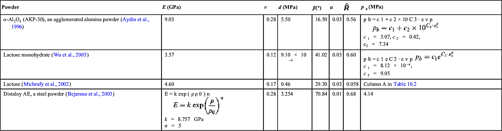
Table 10.2

The Variation of p_b with $ε_{v}^{p}$ $ε_{v}^{p}$ Reported in Michrafy et al. (2002)

p_b (MPa)	$ε_{v}^{p}$ $ε_{v}^{p}$
5.00 × 10⁻⁴	0.20
5.90	0.26
21.51	0.32
19.58	0.37
29.02	0.41
56.64	0.48
97.93	0.55
145.84	0.62
227.72	0.64
239.28	0.65

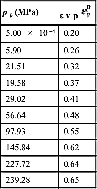
Table 10.3

DPC Parameters for MCC PH 102 from Cunningham et al. (2004): α = 0.03

Relative Density	E (GPa)	v	d (MPa)	β (°)
0.30	0.50	0.02	0.10	41.00	0.05
0.35	0.55	0.03	0.20	46.00	0.08
0.40	0.60	0.04	0.30	48.00	0.11
0.45	0.70	0.05	0.50	52.00	0.13
0.50	0.80	0.07	0.70	54.00	0.16
0.55	0.90	0.08	1.10	57.00	0.20
0.60	1.20	0.10	1.50	58.00	0.25
0.65	2.00	0.12	2.00	61.00	0.32
0.70	2.50	0.14	2.60	63.00	0.39
0.75	3.00	0.17	3.30	65.00	0.45
0.80	4.00	0.20	4.20	66.00	0.51
0.85	4.60	0.23	5.30	68.00	0.58
0.90	6.50	0.26	6.60	71.00	0.65
0.95	8.50	0.29	8.20	72.00	0.75

As an example, consider the compaction of a lactose powder in a die of 8 mm diameter. The calibrated material properties are given in Wu et al. (2005) and are presented in Table 10.1. The powder is compressed with a moving upper punch while the lower punch is stationary. As it is an axisymmetrical problem, it can be modeled with a 2D FEM: only half of the evolving section is meshed using axisymmetric continuum elements. The initial FE mesh is shown in Fig. 10.19(a). The die wall and the upper punch are modeled as rigid bodies since their deformation is negligible compared to that of the powder. The master-slave contact with finite sliding discussed in Section 10.1.1 is employed to model the interaction between the powder and tooling surface. The friction in the contact was determined experimentally using the method described in Section 7.3 and was given in Table 7.1. For the boundary condition, the nodes on the symmetrical axis (AB) are constrained to move in the horizontal direction and the nodes at boundary BC are constrained to move in the vertical direction. The upper punch only moves vertically at a specified compression speed of 3 mm/s. A uniform distribution of the initial relative density is assumed.

Table 10.4

The Variation of p_b with $ε_{v}^{p}$ $ε_{v}^{p}$ for MCC PH 102 from Cunningham et al. (2004): α = 0.03

p_b (MPa)	ε_v
0.043	0
0.62	0.12
1.61	0.26
2.59	0.37
4.08	0.48
6.87	0.57
12.00	0.66
16.80	0.74
23.70	0.81
31.80	0.88
42.30	0.95
56.60	1.01
79.60	1.07
119.00	1.12
143.00	1.14

Table 10.5

DPC Parameters for a steel Powder (Distaloy AE) from Shang et al. (2012)

Relative Density	E (GPa)	v	d (MPa)	β (°)
0.57	9.64	0.19	0.59	71.31	0.48
0.61	13.50	0.16	0.98	70.97	0.48
0.65	15.81	0.16	1.64	70.63	0.50
0.69	19.86	0.15	2.70	70.82	0.52
0.71	22.56	0.15	3.63	70.83	0.53
0.75	30.08	0.14	6.55	70.67	0.56
0.78	37.22	0.12	8.41	70.50	0.58
0.80	39.72	0.12	10.20	70.33	0.60
0.82	45.90	0.12	12.93	70.51	0.62
0.83	51.68	0.11	15.12	69.99	0.63
0.85	55.73	0.11	17.78	70.52	0.65
0.86	60.36	0.11	20.24	70.17	0.67

Table 10.6

The Variation of p_b with $ε_{v}^{p}$ $ε_{v}^{p}$ for a steel Powder (Distaloy AE) from Shang et al. (2012)

p_b (MPa)	ε_v
2.63	0.00
9.33	0.33
18.88	0.42
31.07	0.49
41.52	0.54
54.61	0.59
71.19	0.64
93.89	0.70
111.36	0.74
134.07	0.78
150.68	0.80
172.52	0.83
204.87	0.86
229.35	0.88
250.34	0.90
278.32	0.92
298.44	0.93

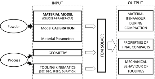
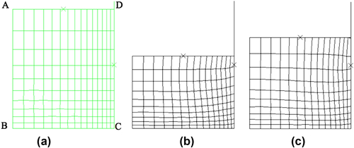
Figure 10.18 Illustration of typical powder compaction modeling process using FEM.

Figure 10.19 Finite element meshes: (a) before compaction, (b) at the end of compression, and (c) during decompression (Wu et al., 2005).

During powder compression, the volume of the powder bed reduces, which manifests itself in the deformation and distortion of the FE meshes as illustrated in Fig. 10.19(b) which shows the FE meshes at the maximum compression. Fig. 10.19(c) shows the meshes at the end of compaction. By examining the FE meshes at different time instants, the deformation of the powder bed is clearly represented: the powder bed is compressed during loading and dilated during unloading (i.e., relaxation). Furthermore, the packing density and stress distributions under the applied pressure can also be determined, which are shown as contour plots in Figs 10.20 and 10.21, respectively.

The density distribution is produced by mapping the relative density of every element. Fig. 10.20 shows the relative density distribution at the maximum compression. It can be seen that the density distribution is not uniform: a high density is induced around the top edge, with a low density at the bottom edge, which is in good agreement with the experimental observations of many others (Train, 1957; Kim, 2003). The nonuniform density distribution is primarily due to the presence of friction at the die wall, which constrains the motion of the powder in that region. Consequently the stress transmitted to the region near the bottom edge is limited and the powder is less compacted there. Near the top edge the powder is subject to a larger stress induced by the combined effect of the compression pressure and the shear stress along the wall, leading to a higher degree of compression and a higher relative density.

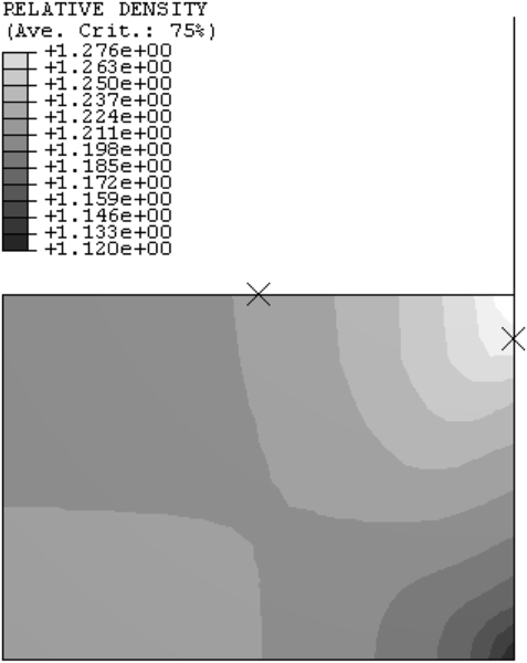
Figure 10.20 Density distribution at maximum compression (Wu et al., 2005).

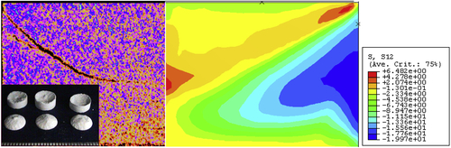
Figure 10.21 The distribution of shear stress obtained using FEM (left), and X-ray computed tomographic images (right) and photographs of ejected lactose tablets (insert) (Wu et al., 2005).

The typical distribution of shear stress at the early stage of the unloading is presented on the right-hand side of Fig. 10.21. It is apparent that there is an intensive localized shear band from the top edge towards the mid-center of the compressed powder. Dilation is generally caused by shear deformation in powders. Consequently, the powder in the shear zone is less compacted and the bonding strength is relatively weak. This is further confirmed by the tablet failure pattern during powder compaction observed from the X-ray tomographic images of the ejected tablet and the photograph of three broken tablets after ejection in the same tests. This experimental evidence shows that cracks are developed from the top edge toward the mid-center, similarly to the pattern of shear banding obtained from the FE analysis. This demonstrates the utility of FE analysis in indicating possible failure patterns during powder compaction. Nevertheless, it remains a challenging task to model and predict the propagation of cracks in compacted products, a task which deserves further study.

..................Content has been hidden....................

You can't read the all page of ebook, please click here login for view all page.

Table of Contents for Chapter 10. Finite Element Modeling

Create new playlist

Sign In

Sign Up

Abstract

Keywords

10.1. Modeling of Particle–Particle Interaction

10.1.1. Contact Modeling Techniques

10.1.2. Applications

10.2. Multiple Particle Finite Element Modeling

10.3. Continuum Modeling of Powder Compaction

10.3.1. Material Models

10.3.2. DPC Model

10.3.3. Determination of Constitutive Properties

10.3.3.1. Young’s modulus E and Poisson’s ratio υ

10.3.3.2. Cohesion d and angle of friction β

10.3.3.4. DPC model calibration procedure

10.3.4. Modeling Procedure and Applications

Table of Contents for
Chapter 10. Finite Element Modeling