Search in book...
Toggle Font Controls
Create new playlist

Name your new playlist

Playlist description (optional)
Sign In

Email address

Password

Forgot Password?

or

Continue with Facebook

Continue with Google
Sign Up

Full Name

Email address

Confirm Email Address

Password

or

Continue with Facebook

Continue with Google

Chapter 4

Particles in Fluids

Abstract

Behavior of a single isolated particle in a fluid: (1) Settling of a single isolated particle in a continuous fluid. (2) Drag force on an isolated particle. (3) Calculation of the terminal velocity. (4) Other shapes. (5) Acceleration and nonsteady motion. (6) Curvilinear motion. (7) Assemblies of particles.

Keywords

Drag; Fluid; Motion; Particle; Particle assemblies; Settling; Terminal velocity

The earlier chapters in this book are mostly concerned with the properties of solid particles, but in particle-processing operations the particles are surrounded by a fluid—a gas or a liquid—or perhaps by a mixture of fluids. Much of particle technology is concerned with the interaction between particles and fluids, which is a vast topic in itself (see, for example, Clift et al., 1978). This chapter concerns only single isolated particles—spheres and other shapes—in a continuous fluid.

4.1. Settling of a Single Isolated Particle in a Continuous Fluid

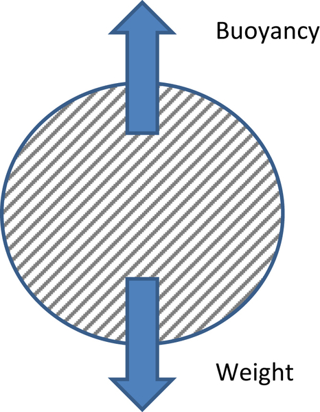
Consider first a single isolated sphere held stationary in a stationary continuous fluid, as shown in Fig. 4.1. What are the forces acting on it?

These are its weight (particle density × particle volume × acceleration due to gravity), and its buoyancy, which according to Archimedes' principle is equal to the weight of fluid displaced (fluid density × particle volume × acceleration due to gravity). Both act vertically.

If the particle is released from rest it will either fall (if its density is above that of the fluid), rise (if the opposite is true), or remain where it is (if the particle and fluid densities are the same). More precisely, if the densities are unequal, weight and buoyancy are unbalanced, and there is a net force on the particle which gives rise to an acceleration. The particle will then move, upward or downward, relative to the fluid, giving rise to a third force, termed the drag force, which acts in the opposite direction to the direction of relative motion. The particle accelerates to its terminal settling velocity, a constant velocity at which the three forces are in balance (Fig. 4.2).

In this condition it is possible to write:

$Drag force = Weight - Buoyancy$ $Drag force = Weight - Buoyancy$

(4.1)

$F_{D} = ρ_{p} g V - ρ g V = (ρ_{p} - ρ) g V$ $F_{D} = ρ_{p} g V - ρ g V = (ρ_{p} - ρ) g V$

(4.2)

where F_D is the drag force, ρ_p and ρ are the densities of the particle and the fluid, respectively, V is the particle volume, and g is the acceleration due to gravity.

Figure 4.1 An isolated stationary sphere in a continuous fluid.

Figure 4.2 An isolated sphere at its terminal settling velocity (particle denser than the fluid).

The question then arises of how to calculate the terminal settling velocity, which should be possible if the drag force is known as a function of particle velocity. (More precisely, this should be relative velocity, since it is the particle velocity relative to that of the fluid which is important. In the case just considered, the fluid is stationary, but in general both the particle and the fluid will be in motion.) Box 4.1 considers how the drag force arises and how it might be calculated.

4.2. Drag Force on an Isolated Particle (Seville et al., 1997)

A relationship between F_D and the terminal velocity u_t is required in order to solve Eq. (4.2), but there is no universally applicable theoretical result for this. It is therefore necessary to use some form of empirical correlation. Such correlations (and there are many available; see Clift et al., 1978) are commonly expressed in terms of two dimensionless variables, the particle Reynolds number,

Box 4.1 A More Complex Situation—Drag, Buoyancy, and Lift on a Nonspherical Shape

Settling of a sphere in a stationary fluid is relatively simple—it is a one-dimensional problem because the forces are all aligned. A much more complex situation is shown in Fig. 4.3, where the particle is nonspherical and the fluid flow direction is not aligned with gravity.

Any element dS of the surface of the particle will experience both a shear stress and a normal stress, acting respectively tangential and normal to the surface. The integral of the shear stress over the surface is the skin friction drag of the fluid on the particle.

The normal stress includes two components: (1) the hydrostatic pressure, whose integral over the surface gives the buoyancy force acting on the particle, which as noted before is equal to the weight of the fluid displaced and acts vertically upward, and (2) the “reduced” pressure caused by the flow, whose integral is known as form drag (The “reduced” pressure represents the difference between the actual pressure in the flowing fluid at dS and the hydrostatic pressure.).

The total drag on the particle, F_D, is the sum of the skin friction drag and the form drag and acts parallel to the fluid approach velocity U. Any component of the total hydrodynamic force normal to U is known as lift.

Figure 4.3 Forces on a stationary particle in a flowing fluid.

${Re}_{p} = ρ U d / μ$ ${Re}_{p} = ρ U d / μ$

(4.3)

and the drag coefficient

$C_{D} = F_{D} / [A (ρ U^{2} / 2)]$ $C_{D} = F_{D} / [A (ρ U^{2} / 2)]$

(4.4)

where A is the cross-sectional area of the particle, and therefore proportional to d². For a spherical particle, A is πd²/4 so that

$C_{D} = 8 F_{D} / π ρ U^{2} d^{2}$ $C_{D} = 8 F_{D} / π ρ U^{2} d^{2}$

(4.5)

Figure 4.4 Drag coefficient C_D as a function of Reynolds number (continuous line—sphere; dashed line—disc with flow parallel to axis; and chain-dashed line—cylinder in cross flow). After Seville et al. (1997).

Experimental data are correlated as C_D = f(Re_p). A simple but reliable expression is due to Turton and Levenspiel (1986):

$C_{D} = \frac{24}{{Re}_{p}} [1 + 0.173 {Re}_{p}^{0.657}] + \frac{0.413}{1 + 16300 {Re}_{p} - 1.09}$ $C_{D} = \frac{24}{{Re}_{p}} [1 + 0.173 {Re}_{p}^{0.657}] + \frac{0.413}{1 + 16300 {Re}_{p} - 1.09}$

(4.6)

which is shown in Fig. 4.4 with corresponding results for a disc with flow parallel to the axis and a cylinder in cross flow (In these two cases, the disc or cylinder diameter is d, and in the case of the cylinder, the drag is calculated per unit length.). Equation (4.6) applies for Re_p < 3 × 10⁵ only, but this covers the range of interest here. Note that C_D goes through a minimum around Re_p = 4000.

As shown in Fig. 4.4, at low Re_p, C_D is inversely proportional to Re_p, while at high Re_p, C_D is approximately constant, and these general observations are true not only of spheres but also of discs and cylinders in these given orientations, with differences in the numerical values.

At low Re_p (Re_p < 1), an exact theoretical result known as Stokes' law applies with

$C_{D} = 24 / {Re}_{p}$ $C_{D} = 24 / {Re}_{p}$

(4.7)

$F_{D} = 3 π μ d U$ $F_{D} = 3 π μ d U$

(4.8)

so that, in this range, the drag force is directly proportional to U.

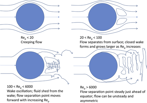
The fluid streamlines are shown schematically in Fig. 4.5. At low Re_p, the particle is described as being in creeping flow, i.e., its motion is dominated by viscous effects in the fluid. Note that according to Eq. (4.8), at low Re_p, the drag force depends on the fluid viscosity but not on its density. Nevertheless, of the total drag at low Re_p, two-thirds arises from the pressure distribution over the sphere and one-third from shear stresses; i.e., even in this creeping flow range, form drag on a sphere is twice the skin friction drag.

The changes in drag coefficient shown in Fig. 4.4 correspond to changes in the fluid flow around the sphere:

• At Re_p = 20, flow separates from the surface to form a closed recirculatory wake which becomes larger as Re_p increases (Fig. 4.5(b)).

• At higher Re_p, the downstream tip of the wake oscillates until, for Re_p > 100, the fluid is shed from the wake. Throughout this range, the point at which flow separates from the surface moves forward with increasing Re_p.

• For Re_p > 6000, the separation point reaches a steady position a little forward of the equator. In this range, skin friction drag is negligible and form drag depends most strongly on the position of flow separation. Therefore, the drag coefficient varies very little with Re_p; over the range 750 < Re_p < 3.4 × 10⁵, C_D only varies by ±13% about a value of 0.445 (or 4/9). This is usually known as the Newton's law range, because Newton's concepts of fluid dynamic drag implied a constant drag coefficient.

Figure 4.5 Flow past a sphere at different Reynolds numbers.

• For Re_p above 10⁵, turbulence intensifies and turbulence bursts occur over the greater part of the surface of the sphere, until a “critical transition” occurs, beyond which the turbulence reattaches and C_D reduces strongly. This range is not usually encountered in particle technology but is important in the behavior of projectiles and balls in sports such as golf.

4.3. Calculation of the Terminal Velocity

Using the drag force relationships above, it is straightforward to calculate the terminal settling velocity, U_t, in the Stokes' law and Newton's law ranges as follows:

For Re_p < 1, from Eqs (4.2) and (4.8),

$F_{D} = (ρ_{p} - ρ) g V = 3 π μ d U_{t}$ $F_{D} = (ρ_{p} - ρ) g V = 3 π μ d U_{t}$

(4.9)

Substituting for V (=πd³/6) and rearranging gives

$U_{t} = d^{2} (ρ_{p} - ρ) g / 18 μ$ $U_{t} = d^{2} (ρ_{p} - ρ) g / 18 μ$

(4.10)

For 10⁴ < Re_p < 2 × 10⁵, Newton's law applies with C_D ≈ 0.445 and from Eq. (4.5)

$U_{t} = 1.73 {[d (ρ_{p} / ρ - 1) g]}^{1 / 2}$ $U_{t} = 1.73 {[d (ρ_{p} / ρ - 1) g]}^{1 / 2}$

(4.11)

In the intermediate regime between the Stokes' and Newton's law ranges, calculation of the terminal velocity is not straightforward because the equations are implicit and iteration is therefore needed. It is therefore preferable to express the drag relationship in a different form:

$U_{t}^{*} = f [d^{*}]$ $U_{t}^{*} = f [d^{*}]$

(4.12)

where

$\begin{matrix} U_{t}^{*} = {[4 {Re}_{t} / 3 C_{D}]}^{1 / 3} \\ = U_{t} {[\frac{ρ^{2}}{μ (ρ_{p} - ρ) g}]}^{1 / 3} \end{matrix}$ $\begin{matrix} U_{t}^{*} = {[4 {Re}_{t} / 3 C_{D}]}^{1 / 3} \\ = U_{t} {[\frac{ρ^{2}}{μ (ρ_{p} - ρ) g}]}^{1 / 3} \end{matrix}$

(4.13)

and

$\begin{matrix} d^{*} = {[3 C_{D} {Re}_{p}^{2} / 4]}^{1 / 3} \\ = d {[\frac{ρ (ρ_{p} - ρ) g}{μ^{2}}]}^{1 / 3} \end{matrix}$ $\begin{matrix} d^{*} = {[3 C_{D} {Re}_{p}^{2} / 4]}^{1 / 3} \\ = d {[\frac{ρ (ρ_{p} - ρ) g}{μ^{2}}]}^{1 / 3} \end{matrix}$

(4.14)

The resulting relationship is shown in Fig. 4.6, and correlations for the full range are tabulated in Table 4.1.

Figure 4.7 shows the terminal velocities of three sizes of particle as functions of temperature at pressures of 1 and 10 bar. The dependence on temperature and pressure illustrates the difference between “small” and “large” particles outlined above. For small particles/low Re_p, the terminal velocity depends on μ but, for particles in gases with ρ << ρ_p, not on ρ; therefore, U_t decreases with increasing temperature but is essentially unaffected by pressure. For relatively large particles/high Re_p, ρ matters but not μ; i.e., the gas flow and the particle motion are dominated by inertial effects, not by viscosity, and the dominant drag term is form drag. The terminal velocity therefore increases as temperature increases (so ρ decreases) but decreases as pressure increases (so ρ increases).

Figure 4.6 The relationship between the dimensionless terminal velocity and dimensionless particle size. After Seville et al. (1997).

Table 4.1

Correlations for Drag and Terminal Velocity (Turton and Levenspiel, 1986; Seville et al., 1997)

1. Spheres a. Drag
Range of Re	Correlation
≤3.38 × 10⁵	$C_{D} = \frac{24}{Re} (1 + 0.173 {Re}^{0.657}) + \frac{0.413}{1 + 1.63 \times 10^{4} {Re}^{- 1.09}}$ $C_{D} = \frac{24}{Re} (1 + 0.173 {Re}^{0.657}) + \frac{0.413}{1 + 1.63 \times 10^{4} {Re}^{- 1.09}}$
3.38 × 10⁵ to 4 × 10⁵	C_D = 29.78 − 5.3 log₁₀ Re
4 × 10⁵ to 10⁶	C_D = 0.1 log₁₀ Re − 0.49
≥10⁶	C_D = 0.19 − 8 × 10⁴ Re⁻¹
b. Free fall or rise Correlations for dimensionless terminal velocity $U_{ts}^{}$ $U_{ts}^{}$ , as a function of dimensionless diameter, d^∗, after Grace (1986). These are defined in Eqs (4.13) and (4.14).

Range of			Correlation
d^∗	U_ts	Re_p	Correlation
≤3.8	≤0.624	≤2.37	$U_{ts}^{} = {(d^{})}^{2} / 18 - 3.1234 \times 10^{- 4} {(d^{})}^{5} + 1.6415 \times 10^{- 6} {(d^{})}^{8} - 7.278 \times 10^{- 10} {(d^{})}^{11}$ $U_{ts}^{} = {(d^{})}^{2} / 18 - 3.1234 \times 10^{- 4} {(d^{})}^{5} + 1.6415 \times 10^{- 6} {(d^{})}^{8} - 7.278 \times 10^{- 10} {(d^{})}^{11}$
3.8–7.58	0.624–1.63	2.37–12.4	x = −1.5446 + 2.9162w − 1.0432w²
7.58–227	1.63–28	12.4–6370	x = −1.64758 + 2.9478w − 1.09703w² + 0.17129w³
226–3500	28–93	6.37 × 10³–3.26 × 10⁵	x = 5.1837 − 4.51034w + 1.687w² − 0.189135w³
Note: w = log₁₀ d^∗; $x = \log_{10} U_{ts}^{}$ $x = \log_{10} U_{ts}^{}$ .
2. $\begin{matrix} Cylinders & E = L / d = aspect ratio \end{matrix}$ $\begin{matrix} Cylinders & E = L / d = aspect ratio \end{matrix}$ a. $\begin{matrix} Drag (E ≫ 1) : C_{D}^{'} = 9.689 {Re}^{- 0.78} \\ \begin{matrix} 0.1 < Re <5 & C_{D} = C_{D}^{'} (1 + 0.147 {Re}^{0.82}) \\ 5 < Re <40 & C_{D} = C_{D}^{'} (1 + 0.227 {Re}^{0.55}) \\ 40 < Re <400 & C_{D} = C_{D}^{'} (1 + 0.0838 {Re}^{0.82}) \end{matrix} \end{matrix}$ $\begin{matrix} Drag (E ≫ 1) : C_{D}^{'} = 9.689 {Re}^{- 0.78} \\ \begin{matrix} 0.1 < Re <5 & C_{D} = C_{D}^{'} (1 + 0.147 {Re}^{0.82}) \\ 5 < Re <40 & C_{D} = C_{D}^{'} (1 + 0.227 {Re}^{0.55}) \\ 40 < Re <400 & C_{D} = C_{D}^{'} (1 + 0.0838 {Re}^{0.82}) \end{matrix} \end{matrix}$ b. $\begin{matrix} Free fall or rise (E \geq 1, d^{} < 20, U_{t}^{} < 25, Re < 100) \\ \log_{10} U_{t}^{} = A_{0} + A_{1} w + A_{2} w^{2} + A_{3} w^{3}, where \\ A_{0} = - 0.66140 - 0.46143 / E - 0.03246 / E^{2} \\ A_{1} = 1.38545 + 1.37542 / E - 0.45526 / E^{2} \\ A_{2} = 0.21234 - 1.27355 / E - 0.57592 / E^{2} \\ A_{3} = - 0.03436 - 0.37525 / E - 0.18969 / E^{2} \end{matrix}$ $\begin{matrix} Free fall or rise (E \geq 1, d^{} < 20, U_{t}^{} < 25, Re < 100) \\ \log_{10} U_{t}^{} = A_{0} + A_{1} w + A_{2} w^{2} + A_{3} w^{3}, where \\ A_{0} = - 0.66140 - 0.46143 / E - 0.03246 / E^{2} \\ A_{1} = 1.38545 + 1.37542 / E - 0.45526 / E^{2} \\ A_{2} = 0.21234 - 1.27355 / E - 0.57592 / E^{2} \\ A_{3} = - 0.03436 - 0.37525 / E - 0.18969 / E^{2} \end{matrix}$

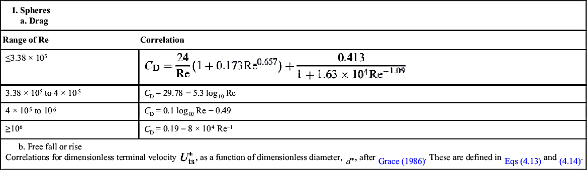
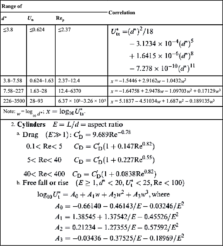
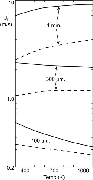
Figure 4.7 Terminal velocity of particles of density 2650 kg/m³ in air (continuous line—1 bar; dashed line—10 bar). After Seville et al. (1997).

4.4. Other Shapes

Figure 4.4 shows the drag–velocity relationships for discs and cylinders as well as spheres, illustrating some interesting effects of shape.

An infinitesimally thin disc in a fluid moving parallel to its axis experiences only form drag because there is no surface parallel to the direction of flow and hence no skin friction. At very low Re_p, this reduces the drag by comparison with a sphere. Wake formation occurs at a lower Re value for a disc, around Re_p = 1, because the sharp edge encourages the flow to separate. Disc wakes start to oscillate at about Re_p = 100 but, because the position of flow separation is fixed, the drag coefficient is constant, at C_D = 1.17, for Re_p > 133. At high Re_p, flow patterns continue to be qualitatively similar to those around a sphere except that, because the separation position is fixed by the particle shape, there is nothing equivalent to the critical transition.

A long cylinder in cross flow shows similar features, but the numerical values of the transitions, such as flow separation, are different. Over the range 70 < Re_p < 2500, wake shedding occurs alternately from the two sides of the cylinder to form a regular series of vortices alternating in their sense of rotation; this is often termed a “von Kármán vortex street.”¹

In order to estimate the drag on a nonspherical particle, it is usual to compare its shape with the standard shapes for which drag coefficient–Reynolds number relationships are known. (The sphere is special in having a unique dimension. The question of how a length dimension is defined for a nonspherical particle is addressed in Chapter 3.) In addition to the sphere, disc, and cylinder, the other common “ideal” shape is the spheroid, which comes in two types: prolate (a sphere distorted by pulling at the poles; a shape like a rugby ball) and oblate (a sphere distorted by pushing at the poles; a shape like a bread bun). Drag relationships for these are given by Clift et al. (1978). In the creeping flow range, the drag on a particle is always less than or equal to that on a body which encloses it and greater than or equal to that on any body contained within it (Hill and Power, 1956). At low Re_p, the drag force is most sensitive to the particle surface, as in the disc–sphere comparison. At intermediate and high Re_p, drag is most likely to be influenced by edges which define the position of flow separation. Such effects can, of course, be reduced by “streamlining,” i.e., profiling the particle shape to prevent boundary layer separation, as in the design of vehicles for high Re number operation.

So far, little mention has been made of orientation. In practice, particles in fluids are usually free to find their own orientation. At Reynolds numbers intermediate between the Stokes' and Newton's law ranges—the range of common practical interest—a nonspherical particle in free motion tends to adopt a preferred orientation with its maximum area presented to the fluid, i.e., in a horizontal plane, for a falling particle. However, particles in gases can maintain other orientations for long times and large distances of travel. The subject of particle orientation is highly complex and dense with studies on different shapes under different conditions. Anyone who has observed leaves falling from trees or coins falling in water will be familiar with some extremes of this behavior. A comprehensive study is presented by Clift et al. (1978).

4.5. Acceleration and Unsteady Motion²

As shown earlier (Eq. (4.10)) the terminal velocity of an isolated particle in free fall under gravity in the Stokes' law range is given by

$U_{t} = τ g$ $U_{t} = τ g$

(4.15)

where

$τ = (ρ_{p} - ρ) d^{2} / 18 μ$ $τ = (ρ_{p} - ρ) d^{2} / 18 μ$

(4.16)

τ is known as the “relaxation time,” so-called because it characterizes the time taken for a particle to adjust to any changes in flow velocity or direction. This approach can be generalized to give the terminal velocity of a particle subjected to any constant external force, F:

$U_{tF} = τ \frac{F}{m}$ $U_{tF} = τ \frac{F}{m}$

(4.17)

During acceleration in a gas, the drag force may still be approximated by Stokes' law, using the instantaneous velocity, so that for acceleration from rest in a gravity field

$m \frac{ⅆ U (t)}{ⅆ t} = m g - 3 π μ U (t) d$ $m \frac{ⅆ U (t)}{ⅆ t} = m g - 3 π μ U (t) d$

(4.18)

$τ \frac{ⅆ U (t)}{ⅆ t} = τ g - U (t)$ $τ \frac{ⅆ U (t)}{ⅆ t} = τ g - U (t)$

(4.19)

which can be solved to give

$U (t) = U_{t} (1 - e^{- t / τ})$ $U (t) = U_{t} (1 - e^{- t / τ})$

(4.20)

By similar reasoning, if U₀ is the initial particle velocity at t = 0 and U_f is the final (steady-state) velocity:

$U (t) = U_{f} - (U_{f} - U_{0}) e^{- t / τ}$ $U (t) = U_{f} - (U_{f} - U_{0}) e^{- t / τ}$

(4.21)

Integrating this equation, the distance traveled, x, can be obtained:

$x (t) = U_{f} t - (U_{f} - U_{0}) τ (1 - e^{- t / τ})$ $x (t) = U_{f} t - (U_{f} - U_{0}) τ (1 - e^{- t / τ})$

(4.22)

In the case of a particle projected into a stagnant gas at velocity U₀, so that U_f = 0, this reduces to

$x (t) = U_{0} τ (1 - e^{- t / τ})$ $x (t) = U_{0} τ (1 - e^{- t / τ})$

(4.23)

so that the “stopping distance” or total distance traveled (for t >> τ) is simply

$x_{s} = U_{0} τ$ $x_{s} = U_{0} τ$

(4.24)

From this, it is now possible to estimate how far a particle can be “thrown” into a stagnant gas. (For a 1 μm particle of density 10³ kg/m³ in air, x_s is about 3.6 μm per (m/s) initial velocity, i.e., a small multiple of its diameter.)

It should be noted that all of the above applies only for particles in gases (or more generally, for particles which are much denser than their surrounding fluid). If this is not the case, as for most particles in liquids, the calculation is more complex (Box 4.2).

Box 4.2 Drag in Unsteady Motion

Earlier sections of this chapter considered steady motion of a particle in a fluid at a constant velocity or under simple acceleration, and it has been shown how dimensional analysis leads to two dimensionless groups, e.g., C_D and Re_p, or d^∗ and

U_{t}^{*}

$U_{t}^{*}$

, which are sufficient to describe the situation completely. In general, unsteady motion is much complex, because the inertia of the particle is important as well as its immersed weight; i.e., ρ_p is significant as well as (ρ_p − ρ). A detailed discussion is given by Clift et al. (1978) but some general points will be summarized here.

In the creeping flow range, the drag on a sphere in unsteady motion through a stagnant fluid can be written

$\begin{matrix} - F_{D} = 3 π μ d U + \frac{1}{2} ρ [\frac{π d^{3}}{6}] \frac{ⅆ U}{ⅆ t} \\ + \frac{3}{2} d^{2} \sqrt{π ρ μ} \int_{- \infty}^{t} {[\frac{ⅆ U}{ⅆ t}]}_{t = s} \frac{ⅆ s}{\sqrt{t - s}} \end{matrix}$ $\begin{matrix} - F_{D} = 3 π μ d U + \frac{1}{2} ρ [\frac{π d^{3}}{6}] \frac{ⅆ U}{ⅆ t} \\ + \frac{3}{2} d^{2} \sqrt{π ρ μ} \int_{- \infty}^{t} {[\frac{ⅆ U}{ⅆ t}]}_{t = s} \frac{ⅆ s}{\sqrt{t - s}} \end{matrix}$

(4.25)

where U(t) is the instantaneous particle velocity.

The total instantaneous drag is made up of three terms, of which the first is the steady (Stokes) drag at the instantaneous velocity. The second term on the right of Eq. (4.25) is known as the “added mass” or “virtual mass” term. It arises from the entrained fluid which accelerates with the particle; for a sphere, this “added mass” of fluid corresponds to a volume equal to half that of the sphere. The final term, known as the “Bassett term” or “history term,” involves an integral over all past accelerations of the sphere. The form of this term arises from the generation of vorticity at the surface of the particle, which diffuses into the surrounding fluid. The history term can be thought of as describing the state of development of the flow around the particle: if it is small, then the relaxation time of the flow is sufficiently small that the instantaneous flow field differs little from steady flow at the instantaneous value of U.

Equation (4.25) can be developed to give an equation of motion of the sphere, for example, to describe the initial motion of a particle released from rest; although its form only applies in creeping flow, it can be extended semiempirically to describe accelerated motion at higher Reynolds numbers; see Clift et al. (1978). Its solution is obviously complicated by the history integral, but some useful general conclusions include:

1. For particles in gases, with ρ_p >> ρ, the added mass and history terms are often small, so that the drag can be approximated by the steady-state drag at the instantaneous velocity. However, this is by no means universally true, even for particles in gases. It is therefore advisable to estimate U(t) by making the quasi-steady approximation and then evaluate the two other terms to verify the validity of the approximation.

2. For particles in liquids, the quasi-steady assumption is almost never justified. Therefore, the kind of calculations made for particles in gases, for example, in inertial devices for separating particles from gases (see Chapter 5), cannot be applied to particles in liquids.

3. The history term is usually larger than the added mass term. Therefore, it is not possible to ignore the history term but to include the added mass term.

4.6. Curvilinear Motion

In the examples considered so far, the forces acting on the particle and the direction of particle motion have all been aligned and the motion has been in a straight line. What happens if particles are subjected to forces acting simultaneously in more than one direction or when there is a change in the direction of the fluid streamlines? A typical example of the latter is when the fluid has to move around an obstacle, such as a fiber in a filter (see Chapter 5). If the fluid is carrying particles with it, will these follow the curving gas streamlines or carry straight on and impact on the obstacle?

Figure 4.8 Path of a particle projected horizontally into a gravity field.

A common example of the case of two forces acting simultaneously in different directions is what happens when a particle is thrown horizontally in a gravitational field, as shown in Fig. 4.8.

This problem is much easier to solve if the motion is at low Re_p, i.e., within the Stokes' regime, because in that case it is possible to analyze the motion independently in the two orthogonal directions. For a particle projected horizontally at a velocity U₀ (from Eq. (4.23)):

$x (t) = U_{0} τ (1 - e^{- t / τ})$ $x (t) = U_{0} τ (1 - e^{- t / τ})$

(4.26)

$y (t) = U_{t} t - U_{t} τ (1 - e^{- t / τ})$ $y (t) = U_{t} t - U_{t} τ (1 - e^{- t / τ})$

(4.27)

If the particle motion is outside the Stokes regime, the motion along one axis affects the motion along other axes and a more complicated analysis is required.

For flow around an obstacle, it is first necessary to define the flow field, using appropriate assumptions, if necessary. The equation of motion of the particle is then solved numerically at successive time intervals (Box 4.3).

4.7. Assemblies of Particles

Only single particles have been considered so far, but what happens if there are many particles. For example, do many particles close together settle at the same settling velocity as a single particle?

Box 4.3 The Stokes Number, St

Curvilinear and other motion of particles in fluids with curved streamlines or of rapidly changing velocity is characterized by the use of a Stokes number, St, which is the ratio of the stopping distance of the particle to a characteristic dimension of the flow, such as a dimension of the obstacle causing the flow disturbance, d_c:

$St = \frac{x_{s}}{d_{c}} = \frac{τ U_{0}}{d_{c}}$ $St = \frac{x_{s}}{d_{c}} = \frac{τ U_{0}}{d_{c}}$

(4.28)

Here U₀ is interpreted as the undisturbed flow (and therefore particle) velocity at infinite distance upstream of the flow disturbance. Thus, the Stokes number can be interpreted as the ratio of the effects of particle inertia to fluid drag, a measure of the tenacity with which particles “hold” to their course rather than following the streamlines. Small values of St indicate good “tracking” of the streamlines, while large values indicate that the particle will “resist” changes in direction or velocity.

An example of the use of the Stokes number in designing cyclones is given in Chapter 5.

In practice, for an assembly of particles the settling velocity is typically much lower than the single-particle terminal velocity. This reduction in settling velocity arises from two complementary effects:

1. The displacement of fluid by the settling particles causes an upflow in the spaces between the particles;

2. The drag on each individual particle is increased by the effect of the neighboring particles on the velocity profile in the interstitial fluid.

Provided that direct particle–particle interactions such as electrostatic forces are negligible, the combined effect is described by the well-known Richardson–Zaki correlation (see Kay and Nedderman, 1985):

$U_{t}^{'} = U_{t} ε^{n}$ $U_{t}^{'} = U_{t} ε^{n}$

(4.29)

where

U_{t}^{'}

$U_{t}^{'}$

and U_t are, respectively, the “hindered settling velocity” and the single-particle terminal velocity, and ε is the void fraction, i.e., (1 − C_v), where C_v is the volumetric concentration of particles. The index n depends on the single-particle Reynolds number, and values are given in Table 4.2. Note that the effect of solids concentration is strongest at the lowest Reynolds number. Equation (4.29) has been shown to describe the expansion of fluidized beds in the nonbubbling mode, as well as sedimentation.

Table 4.2

Values for the Richardson–Zaki Index

Re_p at Terminal Velocity	Value of n
Re_p ≤ 0.2	4.6
0.2 < Re_p < 1	4.4 Re_p^−0.03
1 ≤ Re_p < 500	4.4 Re_p^−0.1
500 ≤ Re_p	2.4

..................Content has been hidden....................

You can't read the all page of ebook, please click here login for view all page.

Table of Contents for Chapter 4. Particles in Fluids

Create new playlist

Sign In

Sign Up

Abstract

Keywords

4.1. Settling of a Single Isolated Particle in a Continuous Fluid

4.2. Drag Force on an Isolated Particle (Seville et al., 1997)

4.3. Calculation of the Terminal Velocity

4.4. Other Shapes

4.5. Acceleration and Unsteady Motion2

4.6. Curvilinear Motion

4.7. Assemblies of Particles

Table of Contents for
Chapter 4. Particles in Fluids

4.5. Acceleration and Unsteady Motion²