Many properties of bulk solids are determined by characteristics of constituent particles, which also influence the behavior of bulk solids during handling and processing. The important characteristics of particles are shape, size, and mechanical properties, such as Young's modulus and Poisson's ratio. From a practical point of view, characterization of particle properties is necessary for product quality control and process monitoring purposes, as the quality of many products is determined by them. In addition, particle characterization also enables a better understanding of the correlation among particle characteristics, process performance, and product quality and also enables improvement in manufacturing efficiency, improves process performance, and increases productivity. It is therefore important to determine these particle characteristics. In this chapter, definitions and measurement methods for particle shape are first briefly introduced. A detailed discussion of particle size characterization is then presented, including the definition of particle size, for which various equivalent diameters are introduced, and various measurement methods. In addition, methods for analysis and presentation of particle size data are explained. Sampling is a critical step in particle shape and size measurement; guidance for sampling both offline and online is presented.
Many properties of bulk solids described in Chapter 2 are determined by the characteristics of their constituent particles, which also influence the behavior of bulk solids during handling and processing. The important characteristics of particles are shape, size, and mechanical properties, such as Young's modulus and Poisson's ratio. There is a plethora of literature demonstrating how particle shape, size, and mechanical properties affect the bulk properties (bulk and tap densities, flowability, compressibility, and compactibility) and their relationship to various processes including flow, packing, compaction, sintering, fluidization, pneumatic conveying, reaction, dissolution, and dispersion. For instance, large and round or blocky particles, such as salt and glass beads, typically flow better than small and irregularly shaped ones like corn flours and chocolate powders, while small particles generally dissolve faster in liquids than large particles but may be more difficult to disperse.
Characterization of particle properties is necessary for product quality control and process monitoring purposes, as the quality of many products is determined by their particle properties. For example, in the pharmaceutical industry, particle size, shape, and mechanical properties affect the dispersion efficiency of dry powder inhalers and the weight and dosage variation of tablets. Particle properties of food and beverage products influence color and flavor. The size and shape of metallic and ceramic particles affect the physical properties of the finished products, such as surface finish and mechanical strength. In process monitoring, control, and optimization, typical applications include crystallization, milling (size reduction), and granulation (size enlargement), for which the aim in each case is to produce particles or granules with desired attributes. Monitoring the change in particle properties (especially size and shape) during the process is therefore critical and requires robust and reproducible characterization.
In addition to quality control and process monitoring, particle characterization enables a better understanding of the correlations between particle characteristics, process performance, and product quality and also enables improvement and optimization of the manufacturing efficiency, improvement in process performance, and increased productivity. In most cases the particle characteristics of interest are difficult to measure, especially for particles smaller than 100μm in size.
3.1. Particle Shape
Particles generally have complex geometric features, summarized under the term shape but including overall form, the presence of reentrant features, and surface irregularity. Shape is therefore difficult to define. Although the literature on particle shape is extensive and a number of shape factors and descriptors are proposed, there is no universal agreement on how to define particle shape and therefore no agreement on how it can be measured properly. Only a small selection of shape factors and descriptors will be discussed in this chapter, but readers are referred to Hawkins (1993) and Endoh (2006) for more comprehensive discussion on the subject.
Particle shapes may be qualitatively characterized by description of their visual appearance, such as spherical, round, angular, dendritic, platy, equidimensional, rodlike, and acicular or needle-shaped. Although these descriptions are simple, easily comprehensible, and convenient to use (Endoh, 2006), they are vague terms that cannot be used to distinguish between particles of similar shapes; quantitative descriptions with clear physical interpretations are needed.
Although many observation methods, such as microscopy, result in a two-dimensional (2D) image, strictly speaking, shape is a three-dimensional (3D) attribute of particles and should be characterized quantitatively based on the analysis of the data in 3D, such as 3D images. Although it is now possible to obtain 3D images of particles of different sizes using advanced imaging techniques, such as X-ray computed tomography (XRCT), it is still problematic and challenging to make 3D measurements and to ensure that the data so obtained are representative. Most particle shape characterization methods are therefore based upon 2D data in the form of projected images obtained using various imaging techniques or sectioned images obtained using metallography or XRCT (Hentschel and Page, 2003). The 2D methods are simple but useful in practice and can to some extent provide representative description of particle shapes as a large number of particles can be projected in random orientations, which provides statistically meaningful information. Therefore, only shape characterization using 2D data will be discussed in this book.
3.1.1. Basic Measurement
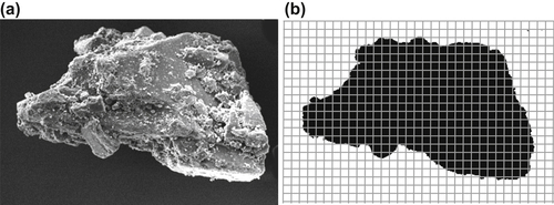
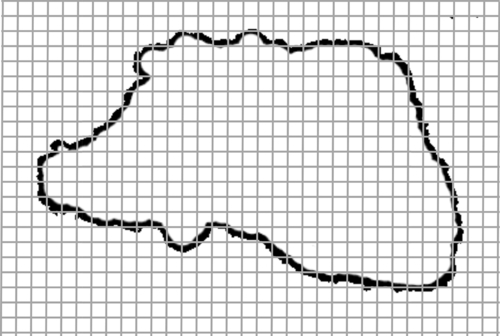
In order to define a shape factor to represent particle shape, some basic measurements of the particle dimensions are needed, which includes length between different boundary features, perimeter, and area. With modern imaging techniques, 2D projected images of particles are normally digitized so that these measurements are generally obtained in the form of pixels, as illustrated in Fig. 3.1, which shows the scanning electron microscopy (SEM) image of a lactose particle and the corresponding projected image used for shape characterization.
Figure 3.1 Scanning electron microscopy (SEM) image of a lactose particle (a) and the corresponding projected image (b).
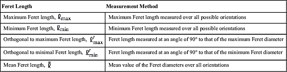
Feret dimensions are the most commonly used length measurements. Feret length ℓ (also known as Feret diameter) is the distance between two tangents to the contour of the particle in a specified direction (see Fig. 3.2). In other words, it corresponds to the measurement by a caliper or slide gauge; hence, it is also called the caliper diameter. Depending on the direction in which the Feret measurement is taken, various Feret lengths can be obtained for the same particle. The commonly used ones are listed in Table 3.1.
The perimeter, P, is the total length of the outline surrounding the projection of the particle, and it is most easily determined by counting the number of boundary pixels (see Fig. 3.3). The area, A, is calculated from the total number of pixels in the particle image (i.e., shaded pixels in Fig. 3.1(b)). It is clear that the accuracy of the perimeter and area measurements is governed by the resolution of the particle images.
Figure 3.2 Feret length of the lactose particle shown in Fig. 3.1 in a random direction.
Maximum Feret length measured over all possible orientations
Minimum Feret length, ℓmin
Minimum Feret length measured over all possible orientations
Orthogonal to maximum Feret length, ℓ′max
Feret length measured at an angle of 90° to that of the maximum Feret diameter
Orthogonal to minimal Feret length, ℓ′min
Feret length measured at an angle of 90° to that of the minimum Feret diameter
Mean Feret length, ℓ¯
Mean value of the Feret diameters over all orientations
Figure 3.3 Perimeter of the lactose particle shown in Fig. 3.1.
3.1.2. Shape Factors
Using the basic measurements discussed in Section 3.1.1, a number of shape factors can be defined. The simplest is the aspect ratio, SA, which is defined as the ratio of the minimum to the maximum Feret length, i.e.,
SA=ℓminℓmax
(3.1)
The aspect ratio is a parameter indicating degree of elongation. A lower value of aspect ratio represents more elongated particles. Another shape factor sensitive to elongation is the roundness, SR:
SR=4πAP2
(3.2)
The roundness typically has a value less than 1. For a perfect sphere (circular projection), SR=1.
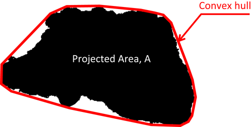
Figure 3.4 Illustration of the circumscribed convex hull for the lactose particle shown in Fig. 3.1.
The sphericity, Ss, is defined as the ratio of the perimeter of the equivalent circle, Pc, to the perimeter of the projection of the particle. The equivalent circle refers to the circle with the same area as the projection of the particle. Hence,
Ss=PcP=2πA√P=SR−−−√
(3.3)
The value of sphericity varies between 0 and 1, for a spherical particle. The more irregular the particle shape is, the smaller the value of sphericity since, for the same projected area, the perimeter increases with increasing departure from a circle.
The convexity SC (also known as solidity) describes the degree of compactness of a particle (Endoh, 2006); it is defined as the ratio of actual area to the area bounded by a convex hull around the projection of the particle (as illustrated in Fig. 3.4), i.e.,
Sc=AAh
(3.4)
where Ah is the area of the circumscribed convex hull. The convexity has a value between 0 and 1, equaling 1 if there are no concave or reentrant features.
3.2. Particle Size
Bulk solids consist of many billions of particles of different size and shape. Determining a distribution of particle size is therefore problematic, since only spheres and cubes can be uniquely defined with a single number such as diameter or the side length. Much theoretical work in particle engineering takes the particles to be spherical but real particles are very rarely spherical. Thus, the use of the term diameter to define the particle size is somehow ambiguous; this difficulty is overcome by use of the concept of equivalent diameter, which is the diameter of a sphere having the same value of a particular physical attribute, such as volume, surface area, or projected area. Many equivalent diameters can be defined, some of which are discussed in this section. Methods for measuring these equivalent diameters and analyzing the resulting data are also introduced. Commercial instruments for particle size characterization may measure different equivalent diameters, as discussed later in this chapter, so that two instruments may not necessarily give exactly the same results for measurements on the same particulate sample. Nevertheless, it is often possible to convert one equivalent diameter to another if some knowledge of the particle shape is available. Conversely, independent measurements of two different equivalent diameters can sometimes be used to infer information about the particle shape.
3.2.1. Particle Size Definition
The equivalent diameters in common use are equivalent project area diameter dA, equivalent surface area diameter dS, equivalent volume diameter dV, Stokes diameter dSt, and aerodynamic diameter da (see Fig. 3.5).
1. Equivalent projected area diameter, dA, is defined as the diameter of a circle with the same area as the projected area of the particle, A, i.e.,
dA=(4Aπ)1/2
(3.5)
Note that for a nonspherical particle, the projected area depends on orientation, as does the equivalent projected area diameter.
2. Equivalent surface area diameter, dS, is the diameter of a sphere with the same surface area, S, as the particle:
dS=(Sπ)1/2
(3.6)
Figure 3.5 Various equivalent diameters for defining the particle size.
3. Equivalent volume diameter, dV, is defined as the diameter of a sphere with the same volume, V, as the particle, i.e.,
dV=(6Vπ)1/3
(3.7)
4. Stokes diameter, dSt, is the diameter of a sphere with the same settling velocity (see Chapter 4) as the particle in the Stokes regime (see section 4.3). Unlike the other definitions introduced above, this equivalent diameter is defined in terms of the aerodynamic behavior of the particle instead of its geometrical properties. It is expressed as
dSt=[18μVtCs(ρp−ρ)g]1/2
(3.8)
where Vt is the particle terminal velocity, Cs is the Cunningham slip correction factor (which can be neglected unless the particles are sub-micron; Seville et al., 1997), μ is the viscosity of the fluid, g is the gravitational acceleration and ρp and ρ are the densities of the particle and the fluid, respectively.
5. Aerodynamic diameter, da, is the diameter of a sphere with a density of 1.0×10³kg/m3 and the same settling velocity as the particle in the Stokes regime. It is similar to the definition of the Stokes diameter given in Eq. (3.8), but instead of using the particle density ρp, it uses a fixed density ρ0=1.0×10³kg/m3, i.e.,
da=[18μVtCa(ρ0−ρ)g]1/2
(3.9)
where Ca is the appropriate Cunningham slip correction factor for da.
As mentioned earlier, it is possible to construct relationships between the different equivalent diameters, which depend on shape. For example, the Stokes diameter can be related to the equivalent volume diameter (Seville et al., 1997):
dSt=[3πd3Vc]1/2
(3.10)
where c is the hydrodynamic resistance of the particle (c=3πd for a sphere). For an irregularly shaped particle, dSt is always greater than dV.
Using Eqs (3.8) and (3.9), it can be shown that the aerodynamic diameter is related to the Stokes diameter as follows
da=ds[Cs(ρp−ρ)Ca(ρ0−ρ)]1/2
(3.11)
For particles in a liquid, Cs=Ca=1, so that Eq. (3.11) becomes
da=ds(ρp−ρρ0−ρ)1/2
(3.12)
For particles in a gas, Cs≈Ca, ρp≫ρ, and ρ0≫ρ, so that Eq. (3.12) reduces to
da=ds(ρpρ0)1/2
(3.13)
The choice of equivalent diameter depends on the actual application, i.e., what the data are intended for. For example, if the separation efficiency of a cyclone is of interest, it is appropriate to use the Stokes diameter, as it best describes the behavior of particles suspended in a fluid. If particle size data are requested for designing dry powder coating processes, the use of the equivalent project area diameter or the equivalent surface area diameter is more appropriate.
3.2.2. Measurement Methods
Many methods and instruments for measuring particle size and concentration have been developed, in response to the increasing demand from researchers and practitioners. Nevertheless, it remains a grand challenge to develop a robust online instrument that has a fast response and can accurately measure the particle size distribution most closely related to the phenomenon under investigation. The purpose of this section is to provide a brief introduction to some common measurement methods for characterizing particle sizes substantially above 1μm, and to explain which equivalent diameter they measure in practice. For sub-micron particles, since the physical laws governing their behavior are generally different, the methods used for measuring the size of these particles form a distinct subject, which will not be considered here.
3.2.2.1. Sieving
As a method of particle separation, a stack of sieves arranged in such a way that mesh sizes decrease with height in the stack can be used to sort particles by size. The powder is placed on the top sieve, and the apparatus is shaken. The powder mass collected in each sieve is then weighed, so that a distribution of the mass of particles with diameters between each sieve size is obtained, and a size distribution by mass can be determined. An advantage of this method is that the sorted fractions can be retained and used for other purposes or for further analysis. In sieving, particles are sorted by the two smallest dimensions (because particles can align to pass through the mesh apertures), so the result may become complex if both size and shape of the particles vary. In practice, an automated sieve shaker is normally used to perform sieving in order to reduce operator bias. Nevertheless, measurement errors can be induced as a result of “blinding” (i.e., sieve blocking), particle breakage (especially for fragile particles), and mesh stretching due to overloading.
3.2.2.2. Microscopy
Particles can be deposited onto a viewing surface and directly observed and measured using either optical microscopy or scanning electron microscopy (SEM). For particles greater than about 10 μm in size, optical microscopy may be sufficient, while SEM is more appropriate for smaller papers, with which high-magnification and high-resolution images can be taken and the size can be measured more accurately. The diameter obtained is the equivalent projected area diameter, dA, in whatever orientation the particles are deposited.
Using this method, as only a limited number of particles can be measured, sampling (see Section 3.3) and preparation are critical to ensure that the selection of particles is representative and each particle can be viewed individually (i.e., to avoid overlap between particle projections). Fortunately, advances in image analysis software enable rapid and automatic data analysis to be performed.
3.2.2.3. Dynamic Image Analysis
The image analysis involved in microscopy discussed above is primarily based on static images, i.e., the images are taken when the sample is stationary. Similar principles can also be applied to analyze dynamic images that are captured when dispersed particles flow past a suitable detector. This is so-called dynamic image analysis.
In dynamic image analysis, particles are dispersed in a gas or liquid and flow past a light source, such as a light-emitting diode (LED). The projection of the particles is then captured with a digital detector (or camera), such as a charge-coupled device and complementary metal-oxide-semiconductor. From the captured images, each particle is identified and analyzed to obtain its size and shape. Similarly to microscopy, dynamic image analysis measures the equivalent projected area diameter.
In most dynamic image analysis systems, a single light source and a single camera are used. Depending on the specification (brightness, focus, resolution) of the light source and camera, only a limited range of particle sizes can be measured. This method has recently been improved by Retsch Technology (Haan, Germany) and the resulting two-camera system is illustrated in Fig. 3.6. This consists of two pulsed LED light sources and two cameras: one camera (i.e., the basic camera in Fig. 3.6) is used to detect large particles and capture more particles in a large-view field so that good statistics can be obtained; the other camera, of high resolution (i.e., the zoom camera), is optimized in order to capture small particles. The two LED light sources are also optimized with appropriate brightness, pulse length, and field of illumination, so that the optical paths of both LED-camera pairs intersect in the measurement area. Using this technique, a wide size range (1μm∼8mm) can be measured with reliable detection of small amounts of small and large particles simultaneously. In addition, the particle shape is also recorded and analyzed for each particle.
Figure 3.6 Principle of dynamic imaging with a two-camera system. Courtesy of Retsch Technology GmbH, reproduced with permission.
3.2.2.4. The Coulter Principle
The Coulter principle, also known as the “electrical sensing zone” or “electrozone” method, is named after its inventor. In this method, particles are dispersed in a weak electrolyte solution that is forced to flow through a small (10–400μm diameter) aperture. On each side of the aperture there is an immersed electrode, between which an electric current can flow (Fig. 3.7), so that an “electric sensing zone” will be created once a voltage is applied across the aperture. When the suspension is sufficiently dilute, particles will pass through the aperture one by one. As each particle goes through the aperture, it displaces its own volume of the conducting liquid and hence changes the electrical resistance across the aperture. With a constant current, the change of impedance generates a voltage pulse whose amplitude is directly proportional to the volume of the conducting liquid being displaced, i.e., the particle volume. As a known volume of particle suspension is drawn through the orifice, the resulting voltage pulses are electronically scaled and registered, from which the number of particles in the suspension can be counted, and a particle size distribution can be determined by scaling the pulse magnitudes in volume units. This method therefore measures the equivalent volume diameter, and the measurement is independent of particle orientation and particle shape. As it counts every single particle, it provides a direct measurement of the particle size distribution.
Figure 3.7 Illustration of the Coulter principle. Courtesy of Beckman Coulter Inc. Reproduced with permission.
The Coulter method requires particles to be well dispersed in the electrolyte, so that an appropriate aqueous or organic electrolyte needs to be used. To establish the correlation between the magnitude of the induced voltage pulse and the particle volume, the instrument must be calibrated using particles of known size, which can be achieved using standard dispersions of polymer latex since the calibration does not need to use the same material as the particles of interest.
3.2.2.5. Aerodynamic Methods
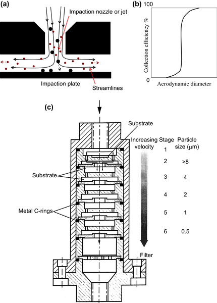
As discussed in detail in Chapter 4 (see also Seville et al., 1997), when dispersed in a fluid, particles of different sizes (and densities) will respond in different ways to any movement of the fluid. This forms the basis of the aerodynamic methods for sizing particles. The inertial impactor is one of the devices that measure particle size using this principle (Fig. 3.8(a)). In the inertial impactor, the gas containing the particles is forced through the impactor nozzle. If an impaction plate is placed close to the nozzle, the jet streamlines bend sharply, as shown. Larger particles, having higher inertia, deviate from the streamlines, impact on the plate, and are collected; small particles are carried away with the gas stream. A typical collection efficiency curve for a single stage of an inertial impactor is illustrated in Fig. 3.8(b), showing the variation of collection efficiency with particle diameter; this is known as a grade efficiency curve.
In practice, a set of inertial impactors is generally stacked to form a cascade impactor (Fig. 3.8(c)), in which the nozzle size is made progressively smaller from stage to stage, resulting in an increase in the jet speed, so that successively smaller particles can be collected and separated on each stage. Particles collected on each impaction plate are weighed so that a size distribution by mass can be obtained. These impactors measure the aerodynamic diameter and are widely used in pharmaceutical and environmental applications, for measuring the particle size distribution of dry powder inhalation formulations and air pollutants, for example.
Figure 3.8 Schematic diagram of (a) an Inertial Impactor and (b) a typical grade efficiency for a single stage of the inertial impactor, and (c) a cascade impactor.
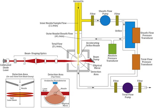
The aerodynamic diameter (or the Stokes diameter) of a particle can be determined by any device that can measure its response to suitably rapid changes in gas velocity. One device based upon this principle is called the aerodynamic particle sizer (APS), manufactured by TSI (Shoreview, MN, USA). In the APS, a suspension of particles flows through a fine nozzle, where the gas is accelerated. Particles suspended in the gas are also accelerated and their rates of acceleration are determined by their aerodynamic size (Fig. 3.9). Large particles accelerate more slowly due to their greater inertia, while fine particles accelerate at a rate closer to that of the gas. When particles leave the nozzle they pass through two closely spaced and partially overlapping laser beams, so that their exit velocities are measured using “time of flight” (Fig. 3.10). Based upon this measurement of individual particle exit velocity, each particle's aerodynamic diameter can be determined and a size distribution can be built up. Similarly to the Coulter method, the APS counts individual particles and provides an absolute measurement of particle size. Although there is a good theoretical basis for the measurement, calibration is still necessary to correlate the measured exit velocity with the particle size, which can be achieved using particles of known size. Furthermore, the suspension entering the instrument must be sufficiently diluted (e.g., by as much as 100:1) to ensure that only one particle is measured at a time.
Figure 3.9 Schematic design of an aerodynamic particle sizer. Courtesy of TSI Inc., MN, USA, www.TSI.com.
Figure 3.10 Illustration of the measuring principle of the aerodynamic particle sizer.
3.2.2.6. Laser Diffraction
Instead of building up a particle size distribution from measurements on individual particles as discussed above, laser diffraction determines the size distribution for the whole sample simultaneously. When a light wave encounters a particle, light is diffracted, the extent of the diffraction depending on its size: large particles scatter light at small angles, while small particles scatter most strongly at large angles. The intensity distribution of the scattered light is usually captured using a multi-element or position-sensitive photo-detector. A laser beam (such as that from a low-power He/Ne laser) is focused into the center of the detector. When particles pass through the laser beam, the scattered light is detected by concentric elements of the detector, and the intensity distribution is then measured. The angular variation in the intensity of scattered light is then analyzed to determine the particle size distribution.
The measured intensity data can be converted mathematically to a particle size distribution using either the Fraunhofer or the more general Mie theory of light scattering, assuming a volume equivalent sphere model (Seville et al., 1997). It is well recognized that the Mie theory provides a better accuracy, especially for measuring small particles, but it requires knowledge of the optical properties (such as the refractive index) of both the sample being measured and the dispersant. The Fraunhofer approximation is a relatively simple approach that does not require knowledge of the optical properties of the sample. It is generally suitable for larger particles (say >10μm).
Laser diffraction can be used to measure particle sizes in suspension in a liquid (i.e., wet) or a gas (i.e., dry) and reports the equivalent volume diameter. The measurement is fast and can be used in situ and for online measurement. Table 3.2 in Box 3.1 summarizes various size measurement methods, the indicative diameter measured, measurement range, and distribution type.
Box 3.1Comparison of Various Size Measurement Methods
Table 3.2
Methods for Particle Size Measurement
Method
Diameter Measured
Range (μm)
Distribution Type
Comments
Sieving
“Sieve diameter”
>20
Mass
Slow; cheap; errors due to blinding, attrition, and fragmentation.
Optical microscopy
dA
0.8–150
Number
Can be interfaced to image analysis computer;
Depth of focus problem; identification possible; chemical analysis possible.
Scanning electronic microscopy
dA
0.01–20
Number
Dynamic imaging analysis
dA
1–3000
Number
Fast; shape determination.
Laser diffraction
dV
0.1–10000
Volume
Fast; online measurement and process control
Aerodynamic (impactor)
dS or da
0.5–50
Mass
Errors due to bounce, breakage; re-entrainment; cheap
Electrozone or Coulter counter
dV
0.3–200
Number
Particles must be dispersed in electrolyte; shape-independent
3.2.3. Size Distribution—Presentation and Analysis
Most powders handled in industrial processes have a wide size distribution, and the fractions of different sized particles vary from batch to batch and from process to process. Powders showing a distribution of particle size are termed polydisperse. For some powders, such as polymer latex spheres formed under zero gravity in industry and plant pollen in nature, the particles are of almost the same size. These powders are termed mondisperse. The following section presents methods for presenting measured particle size data and approaches to describing the particle size distribution.
3.2.3.1. How to Present Particle Size Data
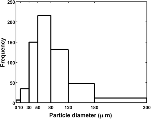
Table 3.3 gives an example of typical particle size data, in which column 4 represents the measured (or “raw”) data. In this example, the sizes of 600 particles are measured and the numbers of particles in discrete size intervals are counted and given as the count frequency. The size distribution is here based on number or count and is therefore a number distribution. Some particle size measurement systems allow the user to specify the limits of the sizing intervals. In this case, it is recommended to keep the resolution (the interval width divided by the mean interval size) approximately constant.
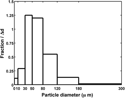
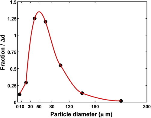
The simplest representation of the size data given in Table 3.3 is a frequency histogram showing the variation of measured count frequency in each size range (Fig. 3.11). It should be noted that this representation can be misleading because the shape of the histogram depends on the choice of the sizing intervals. In order to avoid this problem, it is preferable to divide the count in each interval by the total number of counts to obtain the fraction in each interval (i.e., in each size class, as shown in the 5th column in Table 3.3), and then to divide that fraction by the interval width (usually in micrometers) to obtain the fraction in unit interval width (fraction/μm, see column 6 in Table 3.3). When the fraction/μm is plotted against particle size in a histogram as shown in Fig. 3.12, the resulting representation possesses some unique characteristics: (1) the area under each rectangle represents the fraction of particles in that size interval; and (2) the total area is equal to one. This can be expressed mathematically as follows:
q0(i)=niN=hiΔdi
(3.14)
∑q0(i)=∑iniN=∑i(hiΔdi)=1
(3.15)
where ni is the number of particles in each interval (i.e., particle counts), N is the total number of particles, hi is the height of the ith interval, of width Δdi, and q0(i) is known as the frequency distribution function based on number. q0(i) is defined as the fraction of the total number of particles with diameters between di and di+1 (i.e., the ith interval).
The frequency distribution can be shown either in a discrete form, as in Fig. 3.12, or as a continuous distribution using a smooth curve through q0 (the tops of the frequency rectangles) at the mean value of each interval, as shown in Fig. 3.13. For the mean value of an interval, it is usual to take the geometric mean, i.e., (di·di+1)1/2. However, if the interval width is small, the arithmetic mean, (di+di+1)/2, can be used as these two differ very little. The arithmetic mean is used in Fig. 3.13.
Table 3.3
An Example of a Particle Size Distribution
Size Interval Number, i
Size Range (μm)
Count Frequency
Fraction (Percent in Range), q0(i)
Fraction per μm, q0(i)/Δd
Cumulative Frequency
Cumulative Percent below Upper Bound
Lower
Upper
1
0
20
7
1.17
0.0583
7
1.17
2
20
30
35
5.83
0.5833
42
7.00
3
30
50
150
25.00
1.2500
192
32.00
4
50
80
216
36.00
0.9000
408
68.00
5
80
120
132
22.00
0.5500
540
90.00
6
120
180
48
8.00
0.1333
588
98.00
7
180
300
12
2.00
0.0167
600
100.00
Total
600
100
Figure 3.11 Number frequency distribution.
Figure 3.12 Discrete number distribution: fraction per μm versus particle size.
Figure 3.13 Continuous number distribution: fraction/μm versus particle size.
For a continuous distribution, the fraction of the total number of particles in the size interval [a,b] is given as
qab0=∫abq0(x)ⅆx
(3.16)
where q0(x) is the continuous frequency distribution function based on number. Equation (3.16) indicates that the fraction is the integral under the distribution curve between the limits of the interval. The total area under the distribution curve is again equal to one:
∫0∞q0(x)ⅆx=1
(3.17)
Alternatively, particle size data can also be represented as the cumulative distribution, as shown in Fig. 3.14 for the same data given in Table 3.3. In continuous form, the cumulative number distribution function, Q0(d), is defined as the fraction of the total number of particles with diameters smaller than d:
Q0(d)=∫0dq0(x)ⅆx
(3.18)
or
Figure 3.14 Cumulative number distribution.
q0(x)=ⅆQ(x)0ⅆx
(3.19)
Equation (3.19) shows that the frequency function at any point q0(x) can be determined from the slope of the cumulative distribution function Q0(x).
3.2.3.2. Attributes of a Particle Size Distribution
As shown in Table 3.3 and Section 3.2.3.1, a large amount of information is needed to define a particle size distribution completely. In practice, it is useful to be able to approximate the distribution by some form of mathematical function or by a few (preferably two) parameters that can represent the distribution to some extent, especially for classification and comparison purposes. These functions and parameters are referred to as the characteristics of a particle size distribution. A number of such attributes are introduced for characterizing the particle size distribution, which can be classified into two groups: one for defining the location of the distribution and one for defining its width or breadth. The first group is usually some form of “average,” such as the mean (strictly arithmetic mean), geometric mean, median, or mode:
The arithmetic mean, d¯p, is determined by dividing the sum of all the particle diameters by the total number:
d¯p=∑nidiN
(3.20)
In continuous form, it is given as
d¯p=∫0∞diq0(xi)ⅆxi
(3.21)
The geometric mean, dg, is calculated as follows
dg=[dn11dn22dn33…dnii]1/N
(3.22)
where ni is the number of particles in the ith size class with a diameter of di. In practice, it is more convenient to determine dg by converting Eq. (3.22) to natural logarithms, i.e.,
lndg=∑(nilndi)N
(3.23)
so that
dg=exp[∑(nilndi)N]
(3.24)
The median, often denoted as d50, is the diameter for which 50% of particles are larger, and the other 50% are smaller. It divides the frequency distribution into equal areas (see Fig. 3.13) and is the diameter which corresponds to Q0=0.5 on the cumulative distribution curve (Fig. 3.14). The median is the most frequently used attribute in describing the particle size distribution, as it is less sensitive to skewness (lack of symmetry) of the distribution than the mean.
The mode defines the most frequent size, and it is the size corresponding to the highest point on the frequency curve (see Fig. 3.13).
For distributions that are skewed toward larger sizes as shown in Fig. 3.15, mode < median < mean. In addition to these four averages, it is also possible to define some other attributes that are related to the mass, surface area, or volume of the particles. For example, in Fig. 3.15, the diameter of average mass is defined as the diameter of a sphere of the same average mass as the whole sample, i.e.,
d¯m=[∑nid3iN]1/3
(3.25)
To describe the width or breadth of a particle size distribution, attributes such as variance, quantiles, and span, are introduced. Quantiles are particle size values which divide the distribution such that there is a given proportion below the quantile value. For example, the median divides the distribution such that 50% of the distribution lies below it. Apart from the median, two of the most frequently used quantiles are the lower decile d10, which is defined as the size for which 10% of particles are smaller, and the upper decile d90, which is the diameter for which 90% of the particles are smaller. These can be readily determined from the cumulative size distribution curve (see Fig. 3.14).
Figure 3.15 Illustration of some attributes of the particle size distribution.
The span Ψ is one of the parameters introduced as a measure of the breadth of a distribution and is defined as
Ψ=d90−d10d50
(3.26)
The breadth of a particle size distribution can also be represented by the variance σ2, which is defined as
σ2=∑[q0(d)(d−d¯)2]
(3.27)
where d¯ is the mean and σ is the standard deviation.
3.2.3.3. Weighted Distributions
In many applications, some weighted distribution, such as the distribution by mass or by surface or volume, is more relevant than the number or count distribution discussed so far. For instance, the size distribution of coarse particles is commonly measured using sieving (see Section 3.2.2.1), from which a size distribution by mass (i.e., a mass distribution) is obtained. Just as a number distribution defines the fraction of the total number of particles in any size class, the mass distribution defines the fraction of the total mass of particles in any size class.
It is important to note that, for the same sample, the graphical representations and the values of the attributes for these two distributions are generally different. A product that is 80% by number within a desired size range may contain only 20% of the desired material by weight! Moreover, as discussed in the previous section, measuring instruments may give distributions by number or distributions which are weighted in some way. It is weighted distributions, such as mass, volume, and surface, which are generally of most practical use.
The number mean diameter given in Eq. (3.20) can be rewritten as
d¯p=∑nidiN=∑[niNdi]
(3.28)
Similarly, the mass mean diameter, d¯mm, is given by
d¯mm=∑[miMdi]
(3.29)
where mi is the mass of particles in the ith size class and M is the total mass. The ratio (mi/M) can be regarded as a weighting factor in the averaging process. If particle shape is not a function of particle size, then
mi=kd3i
(3.30)
where k is a constant for all values of di, then
d¯mm=∑[miMdi]=∑midiM=∑nid4i∑nid3i
(3.31)
d¯mm indicates the size of those particles constituting the bulk of the sample volume, so it is also known as the volume moment mean diameter or the mass moment mean diameter. Its value is very sensitive to the presence of large particles.
The surface mean diameter (also known as the “volume–surface mean” or the “Sauter mean”) is defined in a similar way:
d¯sm=∑sidiS=∑nid3i∑nid2i
(3.32)
where si is the surface area of particles in the ith size class and S is the total surface area. The surface mean diameter is often denoted as d¯32 and is the appropriate diameter to use in calculation of the pressure drop through a packed bed of particles at low Reynolds numbers (see Chapters 4 and 5).
In fact, Eqs (3.30) and (3.32) can be further generalized to obtain all the means of a population distribution as follows
d¯a−bab=∑nidai∑nidbi
(3.33)
where a and b are integer variables. Thus, when a=1 and b=0, Eq. (3.33) gives d¯10, that is the number length mean. Similarly
a=2 and b=0 give the number surface mean d¯20;
a=3 and b=0 produce the number volume mean d¯30;
a=3 and b=2 give the surface volume mean d¯32;
a=4 and b=3 give the volume moment mean d¯43;
and so on.
It is possible to represent the same particle size data using different weighted distributions through an appropriate conversion (Box 3.2), which generally requires certain assumptions about the form and physical properties of the particle. The number-based size distribution can also be converted to surface-, mass-, and volume-based size distributions, and vice versa. It is important to note that different weighted distributions are likely to have different attributes (averages, span, etc., see Section 3.2.3.2) even for the same sample or the same particle size data.
Box 3.2Conversion between Weighted Distributions
As an example, let us convert the count size distribution shown in Table 3.3 to a mass distribution. Defining the fraction of the total number of particles in the ith size class as q0(di), the mass of these particles is then
mi=Nq0(di)πd¯3i6ρp
(3.34)
where d¯i is the mean diameter of the size class.
The cumulative mass distribution function Q3(di) is then given by:
where I is the total number of intervals. In fact it is not essential for the particles to be spherical, but only necessary for their shape to be independent of size, i.e., for Eq. (3.30) to be valid. Similarly, to convert a mass distribution, represented by q3(di), to a cumulative number distribution, Q0(di):
Q0(di)=∑i−11[q3(di)d¯3i]∑I1[q3(di)d¯3i]
(3.36)
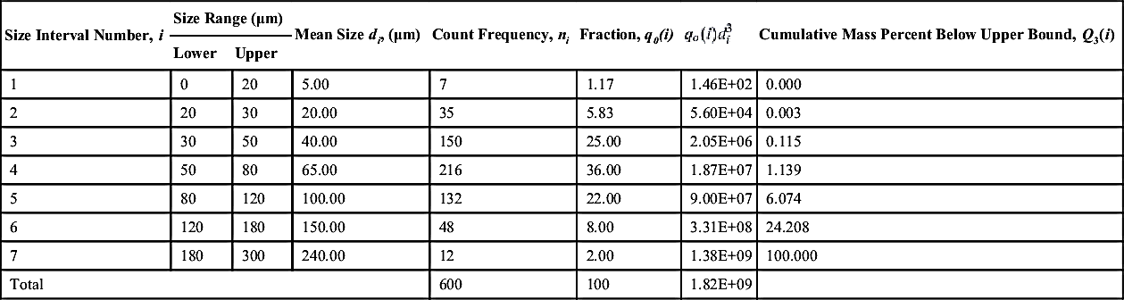
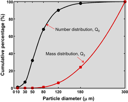
The data of Table 3.3 (showing the number distribution) can now be retabulated to obtain the mass distribution, as shown in Table 3.4. The converted cumulative mass distribution is compared with the measured cumulative number distribution in Fig. 3.16, clearly showing the difference between these two distributions.
Table 3.4
Conversion From Count Distribution to Mass Distribution
Size Interval Number, i
Size Range (μm)
Mean Size di, (μm)
Count Frequency, ni
Fraction, q0(i)
qo(i)d3i
Cumulative Mass Percent Below Upper Bound, Q3(i)
Lower
Upper
1
0
20
5.00
7
1.17
1.46E+02
0.000
2
20
30
20.00
35
5.83
5.60E+04
0.003
3
30
50
40.00
150
25.00
2.05E+06
0.115
4
50
80
65.00
216
36.00
1.87E+07
1.139
5
80
120
100.00
132
22.00
9.00E+07
6.074
6
120
180
150.00
48
8.00
3.31E+08
24.208
7
180
300
240.00
12
2.00
1.38E+09
100.000
Total
600
100
1.82E+09
Figure 3.16 Comparison of converted cumulative mass distribution with the measured cumulative number distribution.
3.3. Sampling for Shape and Size Characterization
Sampling is required for almost all particle characterization techniques before making a measurement, as it is very rare that one can perform a shape-and-size analysis on the entirety of the powder. It is a critical step in characterizing particle shape and size because only a small amount of sample (normally a few grams) is generally needed for the measurement, and the sample needs to be representative of the whole stock or the production stream (kilograms or even tonnes), which is itself often inhomogeneous in time or space or both. Sampling requires careful design and preparation to ensure that the sample is truely representative of the whole. Poorly designed sampling is primarily responsible for unreliable measurements.
Almost all bulk solids are highly polydisperse systems consisting of particles of different sizes, shapes and densities. Due to the differences in these physical properties, the particles tend to segregate (i.e., particles of different properties separate from each other) very easily during transportation and handling. For example, when particles are tipped onto surfaces or into bins, the large particles tend to roll down the sloping sides of the tip, resulting in a greater concentration of fine particles near the center. For powders stored in a container, vibration during transportation may cause smaller particles to sift through the gaps or voids between the large particles, leading to a higher concentration of fines at the bottom of the container. Segregation is therefore the main obstacle in the way of achieving good sampling. A detailed discussion on methods and devices for reliable sampling in these and other circumstances is presented in Allen (1990). Generally a device such as a riffler or sample divider should be used to divide the bulk into many smaller samples that should be further divided using the same technique, in order to obtain a small sample for analysis. Whenever possible, samples should be taken from a moving stream, while the bulk solid is in motion, i.e., before being packed and stored for subsequent usage.
When the powder stream is moving, the following “golden rules” should be followed to achieve appropriate sampling (Allen, 1990): A sample should be taken from the whole powder stream for many equally spaced short periods of time, rather than from part of the stream for the whole time.
When taking samples from a moving powder stream or suspension, two general measurement approaches can be employed: (1) offline measurement, in which the sample is extracted from a moving stream and analyzed outside it, and (2) online measurement, in which the measuring instrument is fitted into the process line and the measurement is carried out in situ. For the offline measurement, the sample is physically contained in the fraction of the total flow that is extracted. For the online measurement, the sample is not physically separated. For example, when optical methods are used, the sample is the fraction of the powder captured by the beam. For both methods, measurements should be taken at different points within the moving stream in order to minimize measurement errors arising from spatial variations in flow velocity and/or particle loading. The advantages and disadvantages of offline and online measurements are compared in Table 3.5.
Table 3.5
Advantages and Disadvantages of Offline and Online Sampling Methods (Seville et al., 1997)
Method
Advantages
Disadvantages
Offline
1. A wide range of equipment can be used;
2. A portion of the sample extracted can be retained;
3. Various analyses can be performed and repeated if necessary.
1. Slow measurement process as the analysis results are not immediately available;
2. The sample may not be representative, as extractive equipment can disturb material flow;
3. Agglomeration may occur in sampling, and conversely de-agglomeration can take place during measurement, resulting in unrepresentative samples for size analysis.
Online
1. Sample extraction equipment is not required;
2. Particles can be monitored as they are being processed;


 (3.5)
(3.5) (3.6)
(3.6)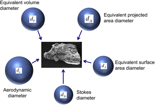
 (3.7)
(3.7) (3.8)
(3.8) (3.9)
(3.9) (3.10)
 (3.11)
 (3.12)
 (3.13)


 (3.16)
 (3.17)
 (3.18)
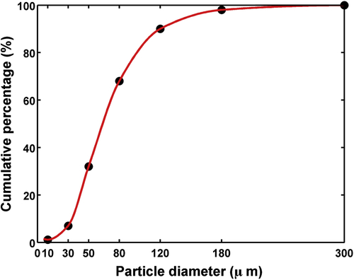
 (3.21)
 (3.25)
 (3.31)
 (3.32)
 (3.35)
 (3.36)