
Chapter 8. Particles
In this chapter we’ll show you how to apply what you’ve learned in Chapter 7 in a simple particle simulator. Before getting to the specifics of the example we’ll present, let’s consider particles in general. Particles are simple idealizations that can be used to simulate all sorts of phenomena or special effects within a game. For example, particle simulations are often used to simulate smoke, fire, and explosions. They can also be used to simulate water, dust clouds, and swarms of insects, among many other things. Really, your imagination is the only limit. Particles lend themselves to simulating both discrete objects like bouncing balls and continua like water. Plus, you can easily ascribe an array of attributes to particles depending on what you’re modeling.
For example, say, you’re modeling fire using particles. Each particle will rise in the air, and as it cools its color will change until it fades away. You can tie the particle’s color to its temperature, which is modeled using thermodynamics. The attribute you’d want to track is the particle’s temperature. In a previous work, AI for Game Programmers (O’Reilly), this book’s coauthor David M. Bourg used particles to represent swarms of insects that would swarm, flock, chase, and evade depending on the artificial intelligence (AI). The AI controlled their behavior, which was then implemented as a system of particles using principles very similar to what you’ll see in this chapter.
Particles are not limited to collections of independent objects either. Later in this book, you’ll learn how to connect particles together using springs to create deformable objects such as cloth. Particles are extremely versatile, and you’ll do well to learn how to leverage their simplicity.
You can use particles to model sand in a simple phone application that simulates an hourglass. Couple this sand model with the accelerometer techniques you’ll learn about in Chapter 21, and you’ll be able to make the sand flow by turning the phone over.
You can easily use particles to simulate bullets flying out of a gun. Imagine a Gatling gun spewing forth a hail of lead, all simulated using simple particles. Speaking of spewing, how about using particles to simulate debris flung from an erupting volcano as a special effect in your adventure game set in prehistoric times? Remember the Wooly Willy toy? To make particles a direct part of game play, consider a diversionary application where you drag piles of virtual magnetic particles around a portrait photograph, giving someone a lovely beard or mustache much like Wooly Willy.
Hopefully, you’re now thinking of creative ways to use particles in your games. So, let’s address implementation. There are two basic ingredients to implementing a particle simulator: the particle model and the integrator. (Well, you could argue that a third basic ingredient is the renderer, where you actually draw the particles, but that’s more graphics than physics, and we’re focusing on modeling and integrating in this book.)
The model very simply describes the attributes of the particles in the simulation along with their rules of behavior. We mean this in the physics sense and not the AI sense in this book, although in general the model you implement may very well include suitable AI rules. Now, the integrator is responsible for updating the state of the particles throughout the simulation. In this chapter, the particles’ states will be described by their position and velocity at any given time. The integrator will update each particle’s state under the influence of several external stimuli—forces such as gravity, aerodynamic drag, and collisions.
The rest of this chapter will walk you through the details of a simple particle simulation in an incremental manner. The first task will be to simulate a set of particles falling under the influence of gravity alone. Even though this sounds elementary, such an example encompasses all of the basic ingredients mentioned earlier. Once gravity is under control, we’ll show you how to implement still air drag and wind forces to influence the particles’ motion. Then, we’ll make things more interesting by showing you how to implement collision response between the particles and a ground plane plus random obstacles. This collision stuff will draw on material presented in Chapter 5, so be sure to read that chapter first if you have not already done so.
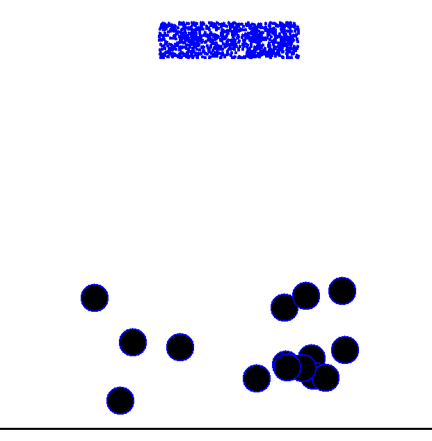
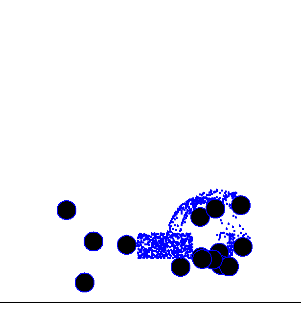
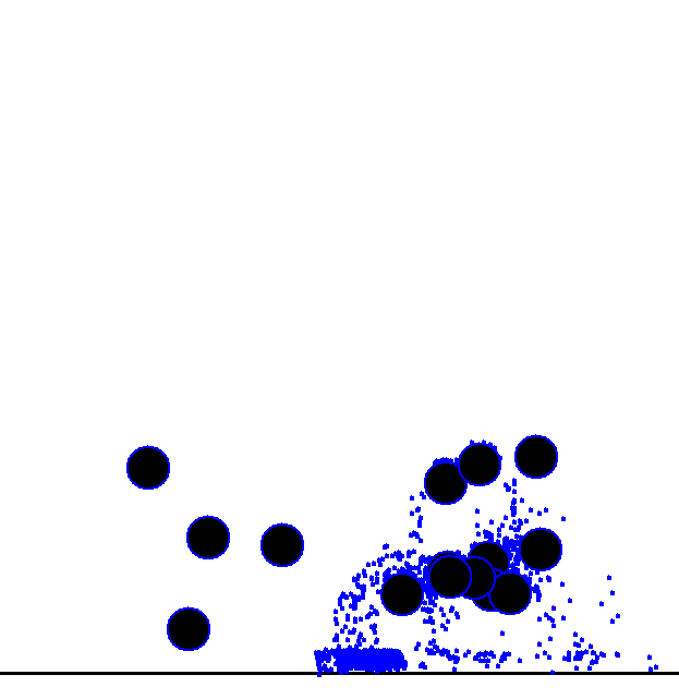
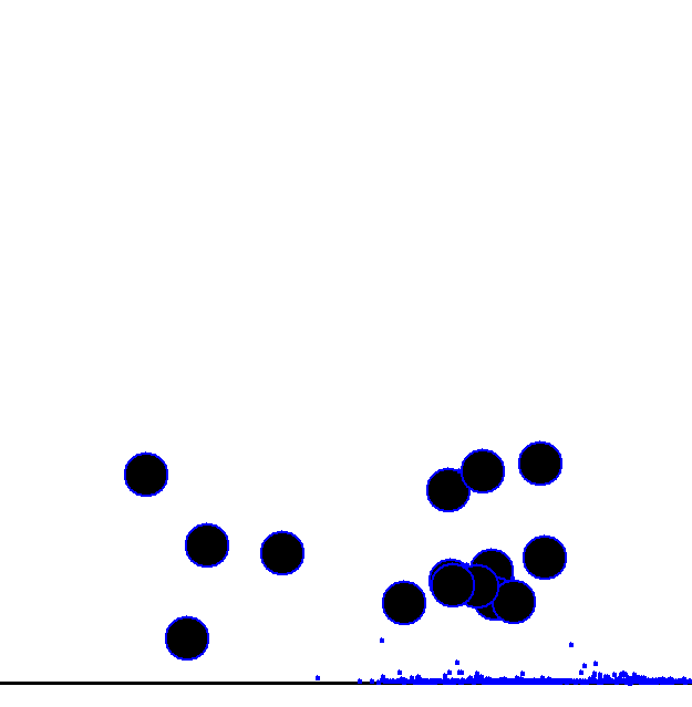
Figure 8-1 through Figure 8-4 show a few frames of this example simulation complete with obstacles and collisions. Use your imagination here to visualize the particles falling under the influence of gravity until they impact the circular objects, at which time they bounce around and ultimately settle on the ground.
While working through this chapter, keep in mind that everything you’re learning here will be directly applicable to 2D and 3D simulations. Chapters following this one will build on the material covered here. We’ll focus on two dimensions in this chapter and later in the book we’ll show you how to extend the simulation to 3D. Actually, for particle simulations it’s almost trivial to make the leap from 2D to 3D. Trust us on this for now.
Simple Particle Model
The particle model we’ll begin with is very simple. All we want to achieve at first is to have the particles fall under the influence of gravity. The particles will be initialized with an altitude above a ground plane. Upon the start of the simulation, gravity will act on each particle, continuously causing each to accelerate toward the ground plane, gaining speed as it goes. Imagine holding a handful of small rocks up high and then releasing them. Simple, huh?
There are several particle attributes we must consider even for this simple example. Our
model assumes that each particle has mass, and a set diameter (we’re assuming our particles
are circles in 2D or spheres in 3D), occupies some position in space, and is traveling at some
velocity. Additionally, each particle is acted upon by some net external force, which is the
aggregate of all forces acting on the particle. These forces will be gravity alone to start
with, but will eventually include drag and impact forces. We set up a Particle class to encapsulate these attributes as follows:
class Particle {
public:
  float   fMass;      // Total mass
  Vector  vPosition;  // Position
  Vector  vVelocity;  // Velocity
  float   fSpeed;     // Speed (magnitude of the velocity)
  Vector  vForces;    // Total force acting on the particle
  float   fRadius;    // Particle radius used for collision detection
  Vector  vGravity;   // Gravity force vector

  Particle(void);     // Constructor
  void  CalcLoads(void);  // Aggregates forces acting on the particle
  void  UpdateBodyEuler(double dt); // Integrates one time step
  void  Draw(void);   // Draws the particle
};
Most of these attributes are self-explanatory given the comments we’ve included. Notice
that several of these attributes are Vector types. These
vectors are defined in the custom math library we’ve included in Appendix A. This type makes managing vectors and performing arithmetic
operations with them a breeze. Take a look at Appendix A to see what
this custom type does. We’ll just remind you of the data structure Vector uses: three scalars called x, y, and
z representing the three dimensions of a location or of a movement in
some direction. The z component will always be set to 0 in this chapter’s
examples.
You should have noticed the fSpeed property in the
Particle class. This property stores the magnitude of the
velocity vector, the particle’s speed. We’ll use this later when computing aerodynamic drag
forces. We’ve also included a Vector type property called
vGravity, which stores the gravity force vector defining
the magnitude and the direction in which the gravity force acts. This is not really necessary,
as you could hardcode the gravity force vector or use a global variable; however, we’ve
included it here to illustrate some creative flexibility. For example, you could redefine the
gravity vector in a game that uses accelerometer input to determine gravity’s direction with respect to a particular
device’s orientation (see Chapter 21). And you may have a game where
some particles react to different gravities depending on their type, which can be of your own
concoction.
Aside from properties, you’ll notice several methods in the Particle class. The constructor is trivial. It sets everything to 0 except the
particle’s mass, radius, and the gravity force vector. The following code illustrates how
everything is initialized:
Particle::Particle(void)
{
  fMass = 1.0;
  vPosition.x = 0.0;
  vPosition.y = 0.0;
  vPosition.z = 0.0;
  vVelocity.x = 0.0;
  vVelocity.y = 0.0;
  vVelocity.z = 0.0;
  fSpeed = 0.0;
  vForces.x = 0.0;
  vForces.y = 0.0;
  vForces.z = 0.0;
  fRadius = 0.1;
  vGravity.x = 0;
  vGravity.y = fMass * _GRAVITYACCELERATION;
}
Now is probably a good time to explain the coordinate system we’ve assumed. Our world origin is located at the lower-left corner of the example program’s window with positive x pointing to the right and positive y pointing up. The acceleration due to gravity acts downward (i.e., in the negative y-direction). We’re using the SI system of units and have defined the acceleration due to gravity as follows:
#define _GRAVITYACCELERATION −9.8f
That’s 9.8 m/s2 in the negative y-direction. We’ve set the mass of each particle to 1 kg by default, which means the force due to gravity is 1 kg times 9.8 m/s2, or 9.8 newtons of force. We’ve set the radius of each particle to one-tenth of a meter. These masses and radii are really arbitrary; you can set them to anything suitable for what you’re modeling.
The CalcLoads method is responsible for computing all
the loads—forces—acting on the particle, with the exception of impact forces (we’ll handle
those later). For now, the only force acting on the particles is that due to gravity, or
simply, the weight of each particle. CalcLoads is very
simple at this point:
void  Particle::CalcLoads(void)
{
  // Reset forces:
  vForces.x = 0.0f;
  vForces.y = 0.0f;

  // Aggregate forces:
  vForces += vGravity;
}
The first order of business is to reset the vForces
vector. vForces is the vector containing the net force
acting on the particle. All of these forces are aggregated in CalcLoads, as shown by the line vForces +=
vGravity. Again, so far, the only force to aggregate is that due to gravity.
Integrator
The UpdateBodyEuler method integrates the equations of motion for each particle. Since we’re dealing with particles, the only equation of
motion we need concern ourselves with is that for translation; rotation does not matter for
particles (at least not for us here). The following code sample shows UpdateBodyEuler.
void Particle::UpdateBodyEuler(double dt)
{
Vector a;
Vector dv;
Vector ds;
// Integrate equation of motion:
a = vForces / fMass;
dv = a * dt;
vVelocity += dv;
ds = vVelocity * dt;
vPosition += ds;
// Misc. calculations:
fSpeed = vVelocity.Magnitude();
}As the name of this method implies, we’ve implemented Euler’s method of integration as described in Chapter 7. Using
this method, we simply need to divide the aggregate forces acting on a particle by the mass
of the particle to get the particle’s acceleration. The line of code a = vForces / fMass does just this. Notice here that a is a Vector, as is vForces. fMass is a scalar,
and the / operator defined in the Vector class takes care of dividing each component of the
vForces vector by fMass and setting the corresponding components in a. The change in velocity, dv, is equal to
acceleration times the change in time, dt. The particle’s
new velocity is then computed by the line vVelocity +=
dv. Here again, vVelocity and dv are Vectors and the
+= operator takes care of the vector arithmetic. This
is the first actual integration.
The second integration takes place in the next few lines, where we determine the
particle’s displacement and new position by integrating its velocity. The line ds = vVelocity * dt determines the displacement, or change in
the particle’s position, and the line vPosition += ds
computes the new position by adding the displacement to the particle’s old position.
The last line in UpdateBodyEuler computes the
particle’s speed by taking the magnitude of its velocity vector.
For demonstration purposes, using Euler’s method is just fine. In an actual game, the more robust method described in Chapter 7 is advised.
Rendering
In this example, rendering the particles is rather trivial. All we do is draw little circles using Windows API calls wrapped in our own functions to hide some of the Windows-specific code. The following code snippet is all we need to render the particles.
void Particle::Draw(void)
{
RECT r;
float drawRadius = max(2, fRadius);
SetRect(&r, vPosition.x − drawRadius,
_WINHEIGHT − (vPosition.y − drawRadius),
vPosition.x + drawRadius,
_WINHEIGHT − (vPosition.y + drawRadius));
DrawEllipse(&r, 2, RGB(0,0,0));
}You can use your own rendering code here, of course, and all you really need to pay close attention to is converting from world coordinates to window coordinates. Remember, we’ve assumed our world coordinate system origin is in the lower-left corner of the window, whereas the window drawing coordinate system has its origin in the upper-left corner of the window. To transform coordinates in this example, all you need to do is subtract the particle’s y-position from the height of the window.
The Basic Simulator
The heart of this simulation is handled by the Particle class
described earlier. However, we need to show you how that class is used in the context of the
main program.
First, we define a few global variables as follows:
// Global Variables: int FrameCounter = 0; Particle Units[_MAX_NUM_UNITS];
FrameCounter counts the number of time steps integrated
before the graphics display is updated. How many time steps you allow the simulation to
integrate before updating the display is a matter of tuning. You’ll see how this is used
momentarily when we discuss the UpdateSimulation function.
Units is an array of Particle types. These will represent moving particles in the simulation—the ones
that fall from above and bounce off the circular objects we’ll add later.
For the most part, each unit is initialized in accordance with the Particle constructor shown earlier. However, their positions are
all at the origin, so we make a call to the following Initialize function to randomly distribute the particles in the upper-middle
portion of the screen within a rectangle of width _SPAWN_AREA_R*4 and a height of _SPAWN_AREA_R,
where _SPAWN_AREA_R is just a global define we made up.
bool Initialize(void)
{
int i;
GetRandomNumber(0, _WINWIDTH, true);
for(i=0; i<_MAX_NUM_UNITS; i++)
{
Units[i].vPosition.x = GetRandomNumber(_WINWIDTH/2-_SPAWN_AREA_R*2,
_WINWIDTH/2+_SPAWN_AREA_R*2, false);
Units[i].vPosition.y = _WINHEIGHT −
GetRandomNumber(_WINHEIGHT/2-_SPAWN_AREA_R,
_WINHEIGHT/2, false);
}
return true;
}OK, now let’s consider UpdateSimulation as shown in the
code snippet that follows. This function gets called every cycle through the program’s main
message loop and is responsible for cycling through all the Units, making appropriate function calls to update their positions, and rendering
the scene.
void UpdateSimulation(void)
{
double dt = _TIMESTEP;
int i;
// initialize the back buffer
if(FrameCounter >= _RENDER_FRAME_COUNT)
{
ClearBackBuffer();
}
// update the particles (Units)
for(i=0; i<_MAX_NUM_UNITS; i++)
{
Units[i].CalcLoads();
Units[i].UpdateBodyEuler(dt);
if(FrameCounter >= _RENDER_FRAME_COUNT)
{
Units[i].Draw();
}
if(Units[i].vPosition.x > _WINWIDTH) Units[i].vPosition.x = 0;
if(Units[i].vPosition.x < 0) Units[i].vPosition.x = _WINWIDTH;
if(Units[i].vPosition.y > _WINHEIGHT) Units[i].vPosition.y = 0;
if(Units[i].vPosition.y < 0) Units[i].vPosition.y = _WINHEIGHT;
}
// Render the scene if required
if(FrameCounter >= _RENDER_FRAME_COUNT) {
CopyBackBufferToWindow();
FrameCounter = 0;
} else
FrameCounter++;
}The two local variables in UpdateSimulation are
dt and i. i is trivial and serves as a counter variable. dt represents the small yet finite amount of time, in seconds,
over which each integration step is taken. The global define_TIMESTEP stores the time step, which we have set to 0.1 seconds. This
value is subject to tuning, which we’ll discuss toward the end of this chapter in the section
Tuning.
The next segment of code checks the value of the frame counter, and if the frame counter
has reached the defined number of frames, stored in _RENDER_FRAME_COUNT, then the back buffer is cleared to prepare it for drawing
upon and ultimately copying to the screen.
The next section of code under the comment update the
particles does just that by calling the CalcLoads and UpdateBodyEuler methods of each
Unit. These two lines are responsible for updating all
the forces acting on each particle and then integrating the equation of motion for each
particle.
The next few lines within the for loop draw each
particle if required and wrap each particle’s position around the window extents should they
progress beyond the edges of the window. Note that we’re using window coordinates in this
example.
Implementing External Forces
We’ll add a couple of simple external forces to start with—still air drag, and wind force. We’ll use the formulas presented in Chapter 3 to approximate these forces, treating them in a similar manner. Recall that still air drag is the aerodynamic drag force acting against an object moving at some speed through still air. Drag always acts to resist motion. While we’ll use the same formulas to compute a wind force, recall that wind force may not necessarily act to impede motion. You could have a tailwind pushing an object along, or the wind could come from any direction with components that push the object sideways. In this example we’ll assume a side wind from left to right, acting to push the particles sideways, with the still air drag resisting their falling motion. When we add collisions later, this same drag formulation will act to resist particle motion in any direction in which they travel as they bounce around.
The formula we’ll use to model still air drag is:
| Fd = ½ ρV2ACd |
Here Fd is the magnitude of the drag force. Its direction is directly opposite the velocity of the moving particle. ρ is the density of air through which the particle moves, V is the magnitude of the particle’s velocity (its speed), A is the projected area of the particle as though it’s a sphere, and Cd is a drag coefficient.
We can use this same formula to estimate the wind force pushing the particle sideways. The only difference this time is that V is the wind speed, and the direction of the resulting wind force is from our assumed left-to-right direction.
To add these two forces to our simulation, we need to make a few additions to the Particle class’s CalcLoads
method. The following code shows how CalcLoads looks now.
Remember, all we had in here originally were the first three lines of executable code shown
next—the code that initializes the aggregate force vector and then the line of code that adds
the force due to gravity to the aggregate force. All the rest of the code in this method is
new.
void Particle::CalcLoads(void)
{
// Reset forces:
vForces.x = 0.0f;
vForces.y = 0.0f;
// Aggregate forces:
// Gravity
vForces += vGravity;
// Still air drag
Vector vDrag;
Float fDrag;
vDrag-=vVelocity;
vDrag.Normalize();
fDrag = 0.5 * _AIRDENSITY * fSpeed * fSpeed *
        (3.14159 * fRadius * fRadius) * _DRAGCOEFFICIENT;
vDrag*=fDrag;
vForces += vDrag;
// Wind
Vector vWind;
vWind.x = 0.5 * _AIRDENSITY * _WINDSPEED *
_WINDSPEED * (3.14159 * fRadius * fRadius) *
_DRAGCOEFFICIENT;
vForces += vWind;
}So after the force due to gravity is added to the aggregate, two new local variables are
declared. vDrag is a vector that will represent the still
air drag force. fDrag is the magnitude of that drag force.
Since we know the drag force vector is exactly opposite to the particle’s velocity vector, we
can equate vDrag to negative vVelocity and then normalize vDrag to obtain a
unit vector pointing in a direction opposite of the particle’s velocity. Next we compute the
magnitude of the drag force using the formula shown earlier. This line handles that:
fDrag = 0.5 * _AIRDENSITY * fSpeed * fSpeed *
(3.14159 * fRadius * fRadius) * _DRAGCOEFFICIENT;Here, _AIRDENSITY is a global define representing the density of air, which we have set to 1.23
kg/m3 (standard air at 15°C). fSpeed is the particle’s speed: the magnitude of its velocity. The 3.14159 * fRadius * fRadius line represents the projected area of
the particle assuming the particle is a sphere. And finally, _DRAGCOEFFICIENT is a drag coefficient that we have set to 0.6. We picked this
value from the chart of drag coefficient for a smooth sphere versus the Reynolds number shown
in Chapter 6. We simply eyeballed a value in the Reynolds number range
from 1e4 to 1e5. You have a choice here of tuning the drag coefficient value to achieve some
desired effect, or you can create a curve fit or lookup table to select a drag coefficient
corresponding to the Reynolds number of the moving particle.
Now that we have the magnitude of the drag force, we simply multiply that force by the
unit drag vector to obtain the final drag force vector. This vector then gets aggregated in
vForces.
We handle the wind force in a similar manner with a few differences in the details. First,
since we know the unit wind force vector is in the positive x-direction (i.e., it acts from
left to right), we can simply set the x component of the wind force
vector, vWind, to the magnitude of the wind force. We
compute that wind force using the same formula we used for still air drag with the exception
of using the wind speed instead of the particle’s speed. We used _WINDSPEED, a global define, to represent the
wind speed, which we have set to 10 m/s (about 20 knots).
Finally, the wind force is aggregated in vForces.
At this stage the particles will fall under the influence of gravity, but not as fast as they would have without the drag force. And now they’ll also drift to the right due to the wind force.
Implementing Collisions
Adding external forces made the simulation a little more interesting. However, to really make it pop, we’re going to add collisions. Specifically, we’ll handle particle-to-ground collisions and particle-to-object collisions. If you have not yet read Chapter 5, which covers collisions, you should because we’ll implement principles covered in that chapter here in the example. We’ll implement enough collision handling in this example to allow particles to bounce off the ground and circular objects, and we’ll come back to collision handling in more detail in Chapter 10. The material in this chapter should whet your appetite. We’ll start with the easier case of particle-to-ground collisions.
Particle-to-Ground Collisions
Essentially what we’re aiming to achieve with particle-to-ground collision detection is to prevent the particles from passing through a ground plane specified at some y coordinate. Imagine a horizontal impenetrable surface that the particles cannot pass through. There are several things we must do in order to detect whether a particle is indeed colliding with the ground plane. If so, then we need to handle the collision, making the particles respond in a suitable manner.
The left side of Figure 8-5 illustrates a collision scenario. It’s easy to determine whether or not a collision has taken place. Over a given simulation time step, a particle may have moved from some previous position (its position at the previous time step) to its current position. If this current position puts the centroid coordinate of the particle within one particle radius of the ground plane, then a collision might be occurring. We say might because the other criteria we need to check in order to determine whether or not a collision is happening is whether or not the particle is moving toward the ground plane. If the particle is moving toward the ground plane and it’s within one radius of the ground plane, then a collision is occurring. It may also be the case that the particle has passed completely through the ground plane, in which case we assume a collision has occurred.
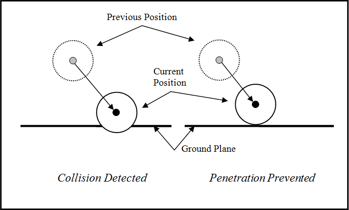
To prevent such penetration of the ground plane, we need to do two things. First, we must reposition the particle so that it is just touching the ground plane, as shown on the right side of Figure 8-5. Second, we must apply some impact force resulting from the collision in order to force the particle to either stop moving down into the ground plane or to move away from the ground plane. All these steps make up collision detection and response.
There are several changes and additions that we must make to the example code in order
to implement particle-to-ground collision detection and response. Let’s begin with the
Particle class.
We’ve added three new properties to Particle, as
follows:
class Particle {
  .
  .
  .
  Vector  vPreviousPosition;
  Vector  vImpactForces;
  bool    bCollision;
  .
  .
  .
};
vPreviousPosition is used to store the particle’s
position at the previous time step—that is, at time t-dt.
vImpactForces is used to aggregate all of the impact
forces acting on a particle. You’ll see later that it is possible for a particle to collide
with more than one object at the same time. bCollision is
simply a flag that is used to indicate whether or not a collision has been detected with the
particle at the current time step. This is important because when a collision occurs, at
that instant in time, we assume that the only forces acting on the particle are the impact
forces; all of the other forces—gravity, drag, and wind—are ignored for that time instant.
We use bCollision in the updated CalcLoads method:
void  Particle::CalcLoads(void)
{
  // Reset forces:
  vForces.x = 0.0f;
  vForces.y = 0.0f;

  // Aggregate forces:
  if(bCollision) {
    // Add Impact forces (if any)
    vForces += vImpactForces;
  } else {
    // Gravity
    vForces += vGravity;

    // Still air drag
    Vector  vDrag;
    float  fDrag;

    vDrag -= vVelocity;
    vDrag.Normalize();
    fDrag = 0.5 * _AIRDENSITY * fSpeed * fSpeed *
           (3.14159 * fRadius * fRadius) * _DRAGCOEFFICIENT;
    vDrag *= fDrag;
    vForces += vDrag;

    // Wind
    Vector  vWind;
    vWind.x = 0.5 * _AIRDENSITY * _WINDSPEED * _WINDSPEED *
             (3.14159 * fRadius * fRadius) * _DRAGCOEFFICIENT;
    vForces += vWind;
  }
}
The only difference between this version of CalcLoads
and the previous one is that we added the conditional if(bCollision) { ... } else { ... }. If bCollision is true, then we have a collision to deal with and the only forces
that get aggregated are the impact forces. If there is no collision, if bCollision is false, then the non-impact forces are aggregated
in the usual manner.
You may have caught that we are aggregating impact forces in this example. This is an alternate approach to the one shown in Chapter 5. There we showed you how to calculate an impulse and change an object’s velocity in response to a collision, using conservation of momentum. Well, we’re still calculating impulses just like in Chapter 5; however, in this example, we’re going to compute the impact force based on that impulse and apply that force to the colliding objects. We’ll let the numerical integrator integrate that force to derive the colliding particle’s new velocities. Either method works, and we’ll show you an example of the former method later. We’re showing the latter method here just to illustrate some alternatives. The advantage of this latter method is that it is easy to compute impact forces due to multiple impacts and let the integrator take care of them all at once.
Now, with these changes made to Particle, we need to
add a line of code to UpdateSimulation, as shown
here:
void  UpdateSimulation(void)
{
  .
  .
  .

  // update computer controlled units:
  for(i=0; i<_MAX_NUM_UNITS; i++)
  {
    Units[i].bCollision = CheckForCollisions(&(Units[i]));
    Units[i].CalcLoads();
    Units[i].UpdateBodyEuler(dt);
    .
    .
    .
  } // end i-loop

  .
  .
  .
}
The new line is Units[i].bCollision =
CheckForCollisions(&(Units[i]));. CheckForCollisions is a new function that takes the given unit, whose pointer
is passed as an argument, and checks to see if it’s colliding with anything—in this case,
the ground. If a collision is detected, CheckForCollisions also computes the impact force and returns true to let us know a collision has occurred. CheckForCollisions is as follows:
bool  CheckForCollisions(Particle* p)
{
  Vector  n;
  Vector  vr;
  float   vrn;
  float   J;
  Vector  Fi;
  bool    hasCollision = false;


    // Reset aggregate impact force
    p->vImpactForces.x = 0;
    p->vImpactForces.y = 0;

    // check for collisions with ground plane
    if(p->vPosition.y <= (_GROUND_PLANE+p->fRadius)) {
      n.x = 0;
      n.y = 1;
      vr = p->vVelocity;
      vrn = vr * n;
      // check to see if the particle is moving toward the ground
      if(vrn < 0.0) {
        J = -(vr*n) * (_RESTITUTION + 1) * p->fMass;
        Fi = n;
        Fi *= J/_TIMESTEP;
        p->vImpactForces += Fi;

        p->vPosition.y = _GROUND_PLANE + p->fRadius;
        p->vPosition.x = ((_GROUND_PLANE + p->fRadius −
                         p->vPreviousPosition.y) /
                        (p->vPosition.y - p->vPreviousPosition.y) *
                        (p->vPosition.x - p->vPreviousPosition.x)) +
                        p->vPreviousPosition.x;

        hasCollision = true;
      }
    }

  return hasCollision;
}
CheckForCollisions makes two checks: 1) it checks to
see whether or not the particle is making contact or passing through the ground plane; and
2) it checks to make sure the particle is actually moving toward the ground plane. Keep in
mind a particle could be in contact with the ground plane right after a collision has been
handled with the particle moving away from the ground. In this case, we don’t want to
register another collision.
Let’s consider the details of this function, starting with the local variables. n is a vector that represents the unit normal vector pointing
from the ground plane to the particle colliding with it. For ground collisions, in this
example, the unit normal vector is always straight up since the ground plane is flat. This
means the unit normal vector will always have an x component of 0 and
its y component will be 1.
The Vector vr is the relative velocity vector between
the particle and the ground. Since the ground isn’t moving, the relative velocity is simply the velocity of the particle. vrn
is a scalar that’s used to store the component of the relative velocity in the direction of
the collision unit normal vector. We compute vrn by
taking the dot product of the relative velocity with the unit normal vector. J is a scalar that stores the impulse resulting from the
collision. Fi is a vector that stores the impact force as
derived from the impulse J. Finally, hasCollision is a flag that’s set based on whether or not a
collision has been detected.
Now we’ll look at the details within CheckForCollisions. The first task is to initialize the impact force vector,
vImpactForces, to 0. Next, we make the first collision
check by determining if the y-position of the particle is less than the ground plane height
plus the particles radius. If it is, then we know a collision may have occurred. (_GROUND_PLANE represents the y coordinate
of the ground plane, which we have set to 100.) If a collision may have occurred, then we
make the next check—to determine if the particle is moving toward the ground plane.
To perform this second check, we compute the unit normal vector, relative velocity, and
relative velocity component in the collision normal direct as described earlier. If the
relative velocity in the normal direction is negative (i.e., if vrn < 0), then a collision has occurred. If either of these checks is
false, then a collision has not occurred and the
function exits, returning false.
The interesting stuff happens if the second check passes. This is where we have to determine the impact force that will cause the particle to bounce off the ground plane. Here’s the specific code that computes the impact force:
        J = -(vr*n) * (_RESTITUTION + 1) * p->fMass;
        Fi = n;
        Fi *= J/_TIMESTEP;
        p->vImpactForces += Fi;

        p->vPosition.y = _GROUND_PLANE + p->fRadius;
        p->vPosition.x = (_GROUND_PLANE + p->fRadius −
                         p->vPreviousPosition.y) /
                        (p->vPosition.y - p->vPreviousPosition.y) *
                        (p->vPosition.x - p->vPreviousPosition.x) +
                         p->vPreviousPosition.x;

        hasCollision = true;
We compute the impulse using the formulas presented in Chapter 5.
J is a scalar equal to the negative of the relative
velocity in the normal direction times the coefficient of restitution plus 1 times the
particle mass. Recall that the coefficient of restitution, _RESTITUTION, governs how elastic or inelastic the collision is, or in other
words, how much energy is transferred back to the particle during the impact. We have this
value set to 0.6, but it is tunable depending on what effect you’re trying to achieve. A
value of 1 makes the particles very bouncy, while a value of, say, 0.1 makes them sort of
stick to the ground upon impact.
Now, to compute the impact force, Fi, that will act
on the particle during the next time step, making it bounce off the ground, we set Fi equal to the collision normal vector. The magnitude of the
impact force is equal to the impulse, J, divided by the
time step in seconds. The line Fi *= J/_TIMESTEP; takes
care of calculating the final impact force.
To keep the particle from penetrating the ground, we reposition it so that it’s just resting on the ground. The y-position is easy to compute as the ground plane elevation plus the radius of the particle. We compute the x-position by linearly interpolating between the particle’s previous position and its current position using the newly computed y-position. This effectively backs up the particle along the line of action of its velocity to the point where it is just touching the ground plane.
When you run the simulation now, you’ll see the particles fall, drifting a bit from left to right until they hit the ground plane. Once they hit, they’ll bounce on the ground, eventually coming to rest. Their specific behavior in this regard depends on what drag coefficient you use and what coefficient of restitution you use. If you have wind applied, when the particles do come to rest, vertically, they should still drift to the right as though they are sliding on the ground plane.
Particle-to-Obstacle Collisions
To make things really interesting, we’ll now add those circular obstacles you saw in Figure 8-1 through Figure 8-4. The particles will be able to hit them
and bounce off or even settle down into crevasses made by overlapping obstacles. The
obstacles are simply static particles. We’ll define them as particles and initialize them
but then skip them when integrating the equations of motion of the dynamic particles. Here’s
the declaration for the Obstacles array:
Particle Obstacles[_NUM_OBSTACLES];
Initializing the obstacles is a matter of assigning them positions and a common radius
and a mass. The few lines of code shown next were added to the main program’s Initialize function to randomly position obstacles in the lower,
middle portion of the window above the ground plane. Figure 8-1 through Figure 8-4 illustrate how they are
distributed.
bool  Initialize(void)
{
  .
  .
  .

  for(i=0; i<_NUM_OBSTACLES; i++)
  {
    Obstacles[i].vPosition.x = GetRandomNumber(_WINWIDTH/2 −
                               _OBSTACLE_RADIUS*10,
                               _WINWIDTH/2 +
                               _OBSTACLE_RADIUS*10, false);
    Obstacles[i].vPosition.y = GetRandomNumber(_GROUND_PLANE +
                               _OBSTACLE_RADIUS, _WINHEIGHT/2 −
                               _OBSTACLE_RADIUS*4, false);
    Obstacles[i].fRadius = _OBSTACLE_RADIUS;
    Obstacles[i].fMass = 100;
  }
  .
  .
  .
}
Drawing the obstacles is easy since they are Particle
types with a Draw method that already draws circular
shapes. We created DrawObstacles to iterate through the
Obstacles array, calling the Draw method of each obstacle.
void DrawObstacles(void)
{
  int    i;

  for(i=0; i<_NUM_OBSTACLES; i++)
  {
    Obstacles[i].Draw();
  }

}
DrawObstacles is then called from UpdateSimulation:
void  UpdateSimulation(void)
{
  .
  .
  .

  // initialize the back buffer
  if(FrameCounter >= _RENDER_FRAME_COUNT)
  {
    ClearBackBuffer();
    // Draw ground plane
    DrawLine(0, _WINHEIGHT - _GROUND_PLANE,
             _WINWIDTH, _WINHEIGHT - _GROUND_PLANE,
             3, RGB(0,0,0));

    DrawObstacles();
  }
  .
  .
  .
}
The last bit of code we need to add to have fully functioning collisions with obstacles
involves adding more collision detection and handling code to the CheckForCollisions function. Before we look at CheckForCollisions, let’s consider colliding circles in general to gain a
better understanding of what the new code will do.
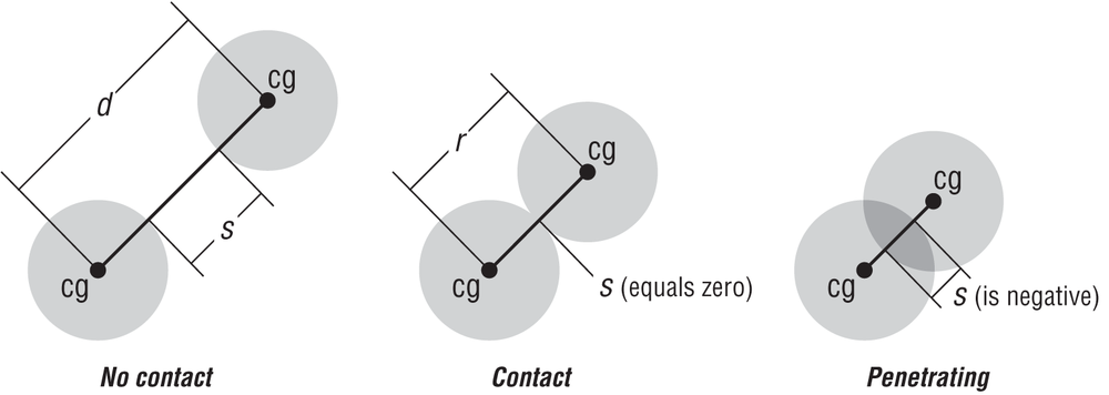
Figure 8-6 illustrates two circles colliding. We aim to detect whether or not these circles are colliding by checking the distance between their centers. If the distance between the two centers is greater than the sum of the radii of the circles, then the particles are not colliding. The topmost illustration in Figure 8-6 shows the distance, d, between centers and the distance, s, between the edges of the circles; s is the gap between the two. Another way to think about this is that if s is positive, then there’s no collision. Referring to the middle illustration in Figure 8-6, if s is equal to 0, then the circles are in contact. If s is a negative number, as shown in the bottommost illustration, then the circles are penetrating.
We’ll apply these principles for detecting colliding circles to detecting collisions between our particles and obstacles since they are both circles. Figure 8-7 illustrates how our particle-to-obstacle collisions might look.
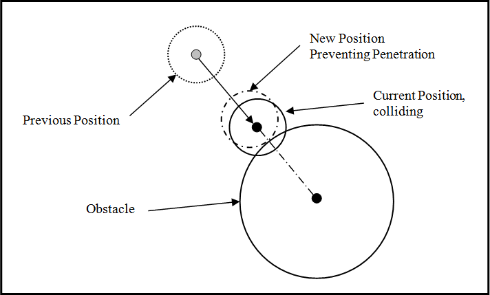
We’ll calculate s for each particle against each obstacle to determine contact or penetration. If we find either, then we’ll perform the relative velocity check in the same manner we did for particle-to-ground collisions to see if the particle is moving toward the obstacle. If it is, then we have a collision and we’ll back up the particle along the collision normal vector line of action, which is simply the line connecting the centers of the particle and the obstacle. We’ll also compute the impact force like we did earlier and let the integrator take care of the rest.
OK, now let’s look at the new code in CheckForCollisions:
bool  CheckForCollisions(Particle* p)
{
  .
  .
  .

    // Check for collisions with obstacles
    float r;
    Vector d;
    float s;

    for(i=0; i<_NUM_OBSTACLES; i++)
    {
      r = p->fRadius + Obstacles[i].fRadius;
      d = p->vPosition - Obstacles[i].vPosition;
      s = d.Magnitude() - r;

      if(s <= 0.0)
      {
        d.Normalize();
        n = d;
        vr = p->vVelocity - Obstacles[i].vVelocity;
        vrn = vr*n;


        if(vrn < 0.0)
        {
          J = -(vr*n) * (_RESTITUTION + 1) /
             (1/p->fMass + 1/Obstacles[i].fMass);
          Fi = n;
          Fi *= J/_TIMESTEP;
          p->vImpactForces += Fi;

          p->vPosition -= n*s;
          hasCollision = true;
        }
      }
    }
  .
  .
  .
}
The new code is nearly the same as the code that checks for and handles particle-to-ground collisions. The only major differences are in how we compute the distance between the particle and the obstacle and how we adjust the colliding particle’s position to prevent it from penetrating an obstacle, since the unit normal vector may not be straight up as it was before. The rest of the code is the same, so let’s focus on the differences.
As explained earlier and illustrated in Figure 8-6, we need to
compute the separation, s, between the particle and the
obstacle. So to get s, we declare a variable r and equate it to the sum of radii of the particle and the
obstacle against which we’re checking for a collision. We define d, a Vector, as the difference between the
positions of the particle and obstacle. The magnitude of d minus r yields s.
If s is less than 0, then we make the relative
velocity check. Now, in this case the collision normal vector is along the line connecting
the centers of the two circles representing the particle and the obstacle. Well, that’s just
the vector d we already calculated. To get the unit
normal vector, we simply normalize d. The relative
velocity vector is simply the difference in velocities of the particle and the obstacle.
Since the obstacles are static, the relative velocity is just the particle’s velocity. But
we calculated the relative velocity by taking the vector difference vr = p->vVelocity – Obstacles[i].vVelocity, because in a more advanced
scenario, you might have moving obstacles.
Taking the dot product of the relative velocity vector, vr, with the unit normal vector yields the relative velocity in the collision
normal direction. If that relative velocity is less than 0, then the particle and the object
are colliding and the code goes on to calculate the impact force in a manner similar to that
described earlier for the particle-to-ground collisions. The only difference here is that
both the particle’s and object’s masses appear in the impulse formula. Earlier we assumed
the ground was infinitely massive relative to the particle’s mass, so the 1/m term for the ground went to 0, essentially dropping out of
the equation. Refer back to Chapter 5 to recall the impulse
formulas.
Once the impact force is calculated, the code backs up the particle by a distance equal
to s, the penetration, along the line of action of the
collision normal vector, giving us what we desire (as shown in Figure 8-7).
Now, when you run this simulation you’ll see the particles falling down, bouncing off the obstacles or flowing around them depending on the value you’re using for coefficient of restitution, ultimately bouncing and coming to rest on the ground plane. If you have a wind speed greater than 0, then the particles will still drift along the ground plane from left to right.
Tuning
Tuning is an important part of developing any simulator. Tuning means different things to different people. For some, tuning is adjusting formulas and coefficients to make your simulation match some specific “right answer,” while to others tuning is adjusting parameters to make the simulation look and behave how you want it to, whether or not it’s technically the right answer. After all, the right answer for a game is that it’s fun and robust. Speaking of robustness, other folks view tuning in the sense of adjusting parameters to make the simulation stable. In reality, this is all tuning and you should think of it as a necessary part of developing your simulation. It’s the process by which you tweak, nudge, and adjust things to make the simulation do what you want it to do.
For example, you can use this same example simulation to model very springy rubber balls. To achieve this, you’ll probably adjust the coefficient of restitution toward a value approaching 1 and perhaps lower the drag coefficient. The particles will bounce all over the place with a lot of energy. If, on the other hand, you want to model something along the lines of mud, then you’ll lower the coefficient of restitution and increase the drag coefficient. There is no right or wrong combination of coefficient of restitution or drag coefficient to use, so long as you are pleased with the results.
Another aspect you might tune is the number of simulation frames per rendering frame. You may find the simulation calculations take so long that your resulting animations are too jerky because you aren’t updating the display enough. The converse may be true in other cases. An important parameter that plays into this is the time step size you take at each simulation iteration. If the step size is too small, you’ll perform a lot of simulation steps, slowing the animation down. On the other hand, a small time step can keep the simulation numerically stable. Your chosen integrator plays a huge role here.
If you make your time step too large, the simulation may just blow up and not work. It will be numerically unstable. Even if it doesn’t blow up, you might see weird results. For example, if the time step in the example simulation discussed in this chapter is too large, then particles may completely step over obstacles in a single time step, missing the collision that would otherwise have happened. (We’ll show you in Chapter 10 how to deal with that situation.)
In general, tuning is a necessary part of developing physics-based simulations, and we encourage you to experiment—trying different combinations of parameters to see what results you can achieve. You should even try combinations that may break the example in this chapter to see what happens and what you should try to avoid in a deployed game.