
Chapter 3. Force
This chapter is a prerequisite to Chapter 4, which addresses the subject of kinetics. The aim here is to provide you with enough of a background on forces so you can readily appreciate the subject of kinetics. This chapter is not meant to be the final word on the subject of force. In fact, we feel that the subject of force is so important to realistic simulations that we’ll revisit it several times in various contexts throughout the remainder of this book. In this chapter, we’ll discuss the two fundamental categories of force and briefly explain some important specific types of force. We’ll also explain the relationship between force and torque.
Forces
As we mentioned in Chapter 2, you need to understand the concept of force before you can fully understand the subject of kinetics. Kinematics is only half the battle. You are already familiar with the concept of force from your daily experiences. You exert a force on this book as you hold it in your hands, counteracting gravity. You exert force on your mouse as you move it from one point to another. When you play soccer, you exert force on the ball as you kick it. In general, force is what makes an object move, or more precisely, what produces an acceleration that changes the velocity. Even as you hold this book, although it may not be moving, you’ve effectively produced an acceleration that cancels the acceleration from gravity. When you kick that soccer ball, you change its velocity from, say, 0 when the ball is at rest to some positive value as the ball leaves your foot. These are some examples of externally applied contact forces.
There’s another broad category of forces, in addition to contact forces, called field forces or sometimes forces at a distance. These forces can act on a body without actually having to make contact with it. A good example is the gravitational attraction between objects. Another example is the electromagnetic attraction between charged particles. The concept of a force field was developed long ago to help us visualize the interaction between objects subject to forces at a distance. You can say that an object is subjected to the gravitational field of another object. Thinking in terms of force fields can help you grasp the fact that an object can exert a force on another object without having to physically touch it.
Within these two broad categories of forces, there are specific types of forces related to various physical phenomena—forces due to friction, buoyancy, and pressure, among others. We’ll discuss idealizations of several of these types of forces in this chapter. Later in this book, we’ll revisit these forces from a more practical point of view.
Before going further, we need to explain the implications of Newton’s third law as introduced in Chapter 1. Remember, Newton’s third law states that for every force acting on a body, there is an equal and opposite reacting force. This means that forces must exist in pairs—a single force can’t exist by itself.
Consider the gravitational attraction between the earth and yourself. The earth is exerting a force—your weight—on you, accelerating you toward its center. Likewise, you are exerting a force on the earth, accelerating it toward you. The huge difference between your mass and the earth’s makes the acceleration of the earth in this case so small that it’s negligible. Earlier we said you are exerting a force on this book to hold it up; likewise, this book is exerting a force on your hands equal in magnitude but opposite in direction to the force you are exerting on it. You feel this reaction force as the book’s weight.
This phenomenon of action-reaction is the basis for rocket propulsion. A rocket engine exerts force on the fuel molecules that are accelerated out of the engine exhaust nozzle. The force required to accelerate these molecules is exerted back against the rocket as a reaction force called thrust. Throughout the remainder of this book, you’ll see many other examples of action-reaction, which is an important phenomenon in rigid-body dynamics. It is especially important when we are dealing with collisions and objects in contact, as you’ll see later.
Force Fields
The best example of a force field or force at a distance is the gravitational attraction between objects. Newton’s law of gravitation states that the force of attraction between two masses is directly proportional to the product of the masses and inversely proportional to the square of the distances separating the centers of each mass. Further, this law states that the line of action of the force of attraction is along the line that connects the centers of the two masses. This is written as follows:
| Fa = (G m1 m2) / r2 |
where G is the gravitational constant, Newton’s so-called universal constant. G was first measured experimentally by Sir Henry Cavendish in 1798 and equals 6.673×10⁻¹¹ (N–m2)/kg2 in metric units or 3.436×10⁻⁸ ft4/(lb-s4) in English units.
So far in this book, I’ve been using the acceleration due to gravity, g, as a constant 9.8 m/s2 (32.174 ft/s2). This is true when you are near the earth’s surface—for example, at sea level. In reality, g varies with altitude—maybe not by much for our purposes, but it does. Consider Newton’s second law along with the law of gravitation for a body near the earth. Equating these two laws, in equation form, yields:
| m a = (G Me m) / (Re + h)2 |
where m is the mass of the body, a is the acceleration of the body due to the gravitational attraction between it and the earth, Me is the earth’s mass, Re is the radius of the earth, and h is the altitude of the body. If you solve this equation for a, you’ll have a formula for the acceleration due to gravity as a function of altitude:
| a = g’ = (G Me) / (Re + h)2 |
The radius of the earth is approximately 6.38×10⁶ m, and its mass is about 5.98×1024 kgs. Substituting these values in the preceding equation and assuming 0 altitude (sea level) yields the constant g that we’ve been using so far—that is, g at sea level equals 9.8 m/s2.
Friction
Frictional forces (friction) always resist motion and are due to the interaction between contacting surfaces. Thus, friction is a contact force. Friction is always parallel to the contacting surfaces at the point of contact—that is, friction is tangential to the contacting surfaces. The magnitude of the frictional force is a function of the normal force between the contacting surfaces and the surface roughness.
This is easiest to visualize by looking at a simple block on a horizontal surface, as shown in Figure 3-1.
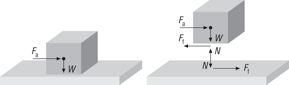
In Figure 3-1, the block is resting on the horizontal surface with a small force, Fa, applied to the block on a line of action through the block’s center of mass. As this applied force increases, a frictional force will develop between the block and the horizontal surface, tending to resist the motion of the block. The maximum value of this frictional force is:
| Ffmax = µs N |
where µs is the experimentally determined coefficient of static[9] friction and N is the normal (perpendicular) force between the block and the surface, which equals the weight of the block in this case. As the applied force increases but is still less than Ffmax, the block will remain static and Ff will be equal in magnitude to the applied force. The block is in static equilibrium. When the applied force becomes greater than Ffmax, the frictional force can no longer impede the block’s motion and the block will accelerate under the influence of the applied force. Immediately after the block starts its motion, the frictional force will decrease from Ffmax to Ffk, where Ffk is:
| Ffk = µk N |
Here k means kinetic since the block is in motion, and µk, the coefficient of kinetic friction,[10] is less than µs. Like the static coefficient of friction, the kinetic coefficient of friction is determined experimentally. Table 3-1 shows typical coefficients of friction for several surfaces in contact.
|
Surface condition |
Μs |
Μu |
% difference |
|
Dry glass on glass |
0.94 |
0.4 |
54% |
|
Dry iron on iron |
1.1 |
0.15 |
86% |
|
Dry rubber on pavement |
0.55 |
0.4 |
27% |
|
Dry steel on steel |
0.78 |
0.42 |
46% |
|
Dry Teflon on Teflon |
0.04 |
0.04 |
— |
|
Dry wood on wood |
0.38 |
0.2 |
47% |
|
Ice on ice |
0.1 |
0.03 |
70% |
|
Oiled steel on steel |
0.10 |
0.08 |
20% |
The data in Table 3-1 is provided here to show you the magnitude of some typical friction coefficients and the relative difference between the static and kinetic coefficients for certain surface conditions. Other data is available for these and other surface conditions in the technical literature (see the Bibliography for sources). Note that experimentally determined friction coefficient data will vary, even for the same surface conditions, depending on the specific condition of the material used in the experiments and the execution of the experiment itself.
Fluid Dynamic Drag
Fluid dynamic drag forces oppose motion like friction. In fact, a major component of fluid dynamic drag is friction that results from the relative flow of the fluid over (and in contact with) the body’s surface. Friction is not the only component of fluid dynamic drag, though. Depending on the shape of the body, its speed, and the nature of the fluid, fluid dynamic drag will have additional components due to pressure variations in the fluid as it flows around the body. If the body is located at the interface between two fluids (like a ship on the ocean where the two fluids are air and water), an additional component of drag will exist due to the wave generation.
In general, fluid dynamic drag is a complicated phenomenon that is a function of several factors. We won’t go into detail in this section on all these factors, since we’ll revisit this subject later. However, we do want to discuss how the viscous (frictional) component of these drag forces is typically idealized.
Ideal viscous drag is a function of velocity and some experimentally determined drag coefficient that’s supposed to take into account the surface conditions of the body, the fluid properties (density and viscosity), and the flow conditions. You’ll typically see a formula for viscous drag force in the form:
| Fv = –Cf v |
where Cf is the drag coefficient, v is the body’s speed, and the minus sign means that the force opposes motion. This formula is valid for slow-moving objects in a viscous fluid. “Slow moving” implies that the flow around the body is laminar, which means that the flow streamlines are undisturbed and parallel.
For fast-moving objects, you’ll use the formula for Fv written as a function of speed squared as follows:
| Fv = –Cf v2 |
“Fast moving” implies that the flow around the object is turbulent, which means that the flow streamlines are no longer parallel and there is a sort of mixing effect in the flow around the object. Note that the values of Cf are generally not the same for these two equations. In addition to the factors mentioned earlier, Cf depends significantly on whether the flow is laminar or turbulent.
Both of these equations are very simplified and inadequate for practical analysis of fluid flow problems. However, they do offer certain advantages in computer game simulations. Most obviously, these formulas are easy to implement—you need only know the velocity of the body under consideration, which you get from your kinematic equations, and an assumed value for the drag coefficient. This is convenient, as your game world will typically have many different types of objects of all sizes and shapes that would make rigorous analysis of each of their drag properties impractical. If the illusion of realism is all you need, not real-life accuracy, then these formulas may be sufficient.
Another advantage of using these idealized formulas is that you can tweak the drag coefficients as you see fit to help reduce numerical instabilities when solving the equations of motion, while maintaining the illusion of realistic behavior. If real-life accuracy is what you’re going for, then you’ll have no choice but to consider a more involved (read: complicated) approach for determining fluid dynamic drag. We’ll talk more about drag in Chapter 6 through Chapter 10.
Pressure
Many people confuse pressure with force. You have probably heard people say, when explaining a phenomenon, something like, “It pushed with a force of 100 pounds per square inch.” While you understand what they mean, they are technically referring to pressure, not force. Pressure is force per unit area, thus the units pounds per square inch (psi) or pounds per square foot (psf) and so on. Given the pressure, you’ll need to know the total area acted on by this pressure in order to determine the resultant force. Force equals pressure times area:
| F = PA |
This formula tells you that for constant pressure, the greater the area acted upon, the greater the resultant force. If you rearrange this equation solving for pressure, you’ll see that pressure is inversely proportional to area—that is, the greater the area for a given applied force, the smaller the resulting pressure and vice versa.
| P = F/A |
An important characteristic of pressure is that it always acts normally (perpendicularly) to the surface of the body or object it is acting on. This fact gives you a clue as to the direction of the resultant force vector.
We wanted to mention pressure here because you’ll be working with it to calculate forces when you get to the chapters in this book that cover the mechanics of ships, boats, and hovercraft. There, the pressures that you’ll consider are hydrostatic pressure (buoyancy) and aerostatic lift. We’ll take a brief look at buoyancy next.
Buoyancy
You’ve no doubt felt the effects of buoyancy when immersing yourself in the bathtub. Buoyancy is why you feel lighter in water than you do in air and why some people can float on their backs in a swimming pool.
Buoyancy is a force that develops when an object is immersed in a fluid. It’s a function of the volume of the object and the density of the fluid and results from the pressure differential between the fluid just above the object and the fluid just below the object. Pressure increases the deeper you go in a fluid, thus the pressure is greater at the bottom of an object of a given height than it is at the top of the object. Consider the cube shown in Figure 3-2.
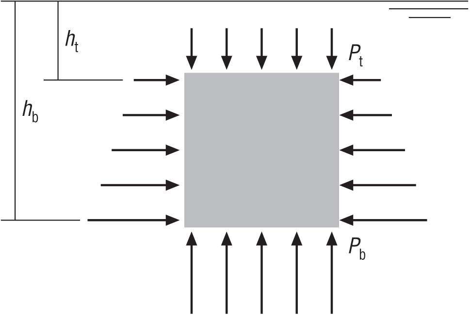
Let s denote the cube’s length, width, and height, which are all equal. Further, let ht denote the depth to the top of the cube and hb the depth to the bottom of the cube. The pressure at the top of the cube is Pt = ρ g ht, which acts over the entire surface area of the top of the cube, normal to the surface in the downward direction. The pressure at the bottom of the cube is Pb = ρ g hb, which acts over the entire surface area of the bottom of the cube, normal to the surface in the upward direction. Note that the pressure acting on the sides of the cube increases linearly with submergence, from Pt to Pb. Also, note that since the side pressure is symmetric, equal and opposite, the net side pressure is 0, which means that the net side force (due to pressure) is also 0. The same is not true of the top and bottom pressures, which are obviously not equal, although they are opposite.
The force acting down on the top of the cube is equal to the pressure at the top of the cube times the surface area of the top. This can be written as follows:
| Ft = Pt At |
| Ft = (ρ g ht) (s2) |
Similarly, the force acting upward on the bottom of the cube is equal to the pressure at the bottom times the surface area of the bottom.
| Fb = Pb Ab |
| Fb = (ρ g hb) (s2) |
The net vertical force (buoyancy) equals the difference between the top and bottom forces:
| FB = Fb – Ft |
| FB = (ρ g hb) (s2) – (ρ g ht) (s2) |
| FB = (ρ g) (s2) (hb – ht) |
This formula gives the magnitude of the buoyancy force. Its direction is straight up, counteracting the weight of the object.
There is an important observation we need to make here. Notice that (hb – ht) is simply the height of the cube, which is s in this case. Substituting s in place of (hb – ht) reveals that the buoyancy force is a function of the volume of the cube.
| FB = (ρ g) (s3) |
This is great since it means that all you need to do in order to calculate buoyancy is to first calculate the volume of the object and then multiply that volume by the specific weight[11] (ρ g) of the fluid. In truth, that’s a little easier said than done for all but the simplest geometries. If you’re dealing with spheres, cubes, cylinders, and the like, then calculating volume is easy. However, if you’re dealing with any arbitrary geometry, then the volume calculation becomes more difficult. There are two ways to handle this difficulty. The first way is to simply divide the object into a number of smaller objects of simpler geometry, calculate their volumes, and then add them all up. The second way is to use numerical integration techniques to calculate volume by integrating over the surface of the object.
You should also note that buoyancy is a function of fluid density, and you don’t have to be in a fluid as dense as water to experience the force of buoyancy. In fact, there are buoyant forces acting on you right now, although they are very small, due to the fact that you are immersed in air. Water is many times more dense than air, which is why you notice the force of buoyancy when in water and not in air. Keep in mind, though, that for very light objects with relatively large volumes, the buoyant forces in air may be significant. For example, consider simulating a large balloon.
Springs and Dampers
Springs are structural elements that, when connected between two objects, apply equal and opposite forces to each object. This spring force follows Hooke’s law and is a function of the stretched or compressed length of the spring relative to the rest length of the spring and the spring constant of the spring. Hooke’s law states that the amount of stretch or compression is directly proportional to the force being applied. The spring constant is a quantity that relates the force exerted by the spring to its deflection:
| Fs = ks (L – r) |
Here, Fs is the spring force, ks is the spring constant, L is the stretched or compressed length of the spring, and r is the rest length of the spring. In the metric system of units, Fs would be measured in newtons (1 N = 1 kg-m/s2), L and r in meters, and ks in kg/s2. If the spring is connected between two objects, it exerts a force of Fs on one object and –Fs on the other; these are equal and opposite forces.
Dampers are usually used in conjunction with springs in numerical simulations. They act like viscous drag in that they act against velocity. In this case, if the damper is connected between two objects that are moving toward or away from each other, the damper acts to slow the relative velocity between the two objects. The force developed by a damper is proportional to the relative velocity of the connected objects and a damping constant, kd, that relates relative velocity to damping force.
| Fd = kd (v1 – v2) |
This equation shows the damping force, Fd, as a function of the damping constant and the relative velocity of the connected points on the two connected bodies. In metric units, where the damping force is measured in newtons and velocity in m/s, kd has units of kg/s.
Typically, springs and dampers are combined into a single spring-damper element, where a single formula represents the combined force. Using vector notation, we can write the formula for a spring-damper element connecting two bodies as follows:
| F1 = –{ks (L – r) + kd ((v1 – v2) • L)/L} L/L |
Here, F1 is the force exerted on body 1, while the force, F2, exerted on body 2 is:
| F2 = –F1 |
L is the length of the spring-damper (L, not in bold print, is the magnitude of the vector L), which is equal to the vector difference in position between the connected points on bodies 1 and 2. If the connected objects are particles, then L is equal to the position of body 1 minus the position of body 2. Similarly, v1 and v2 are the velocities of the connected points on bodies 1 and 2. The quantity (v1 – v2) represents the relative velocity between the connected bodies.
Springs and dampers are useful when you want to simulate collections of connected particles or rigid bodies. The spring force provides the structure, or glue, that holds the bodies together (or keeps them separated by a certain distance), while the damper helps smooth out the motion between the connected bodies so it’s not too jerky or springy. These dampers are also very important from a numerical stability point of view in that they help keep your simulations from blowing up. We’re getting a little ahead of ourselves here, but we’ll show you how to use these spring-dampers in real-time simulations in Chapter 13.
Force and Torque
We need to make the distinction here between force and torque.[12] Force is what causes linear acceleration, while torque is what causes rotational acceleration. Torque is force times distance. Specifically, to calculate the torque applied by a force acting on an object, you need to calculate the perpendicular distance from the axis of rotation to the line of action of the force and then multiply this distance by the magnitude of the force.
This calculation gives the magnitude of the torque. Typical units for force are pounds, newtons, and tons. Since torque is force times a distance, its units take the form of a length unit times a force unit (e.g., foot-pounds, newton-meters, or foot-tons).
Since both force and torque are vector quantities, you must also determine the direction of the torque vector. The force vector is easy to visualize: its line of action passes through the point of application of the force, with its direction determined by the direction in which the force is applied. As a vector, the torque’s line of action is along the axis of rotation, with the direction determined by the direction of rotation and the right hand rule (see Figure 3-3). As noted in Chapter 2, the right hand rule is a simple trick to help you keep track of vector directions—in this case, the torque vector. Pretend to curl the fingers of your right hand around the axis of rotation with your fingertips pointing in the direction of rotation. Now extend your thumb, as though you are giving a thumbs up, while keeping your fingers curled around the axis. The direction that your thumb is pointing indicates the direction of the torque vector. Note that this makes the torque vector perpendicular to the applied force vector, as shown in Figure 3-3.
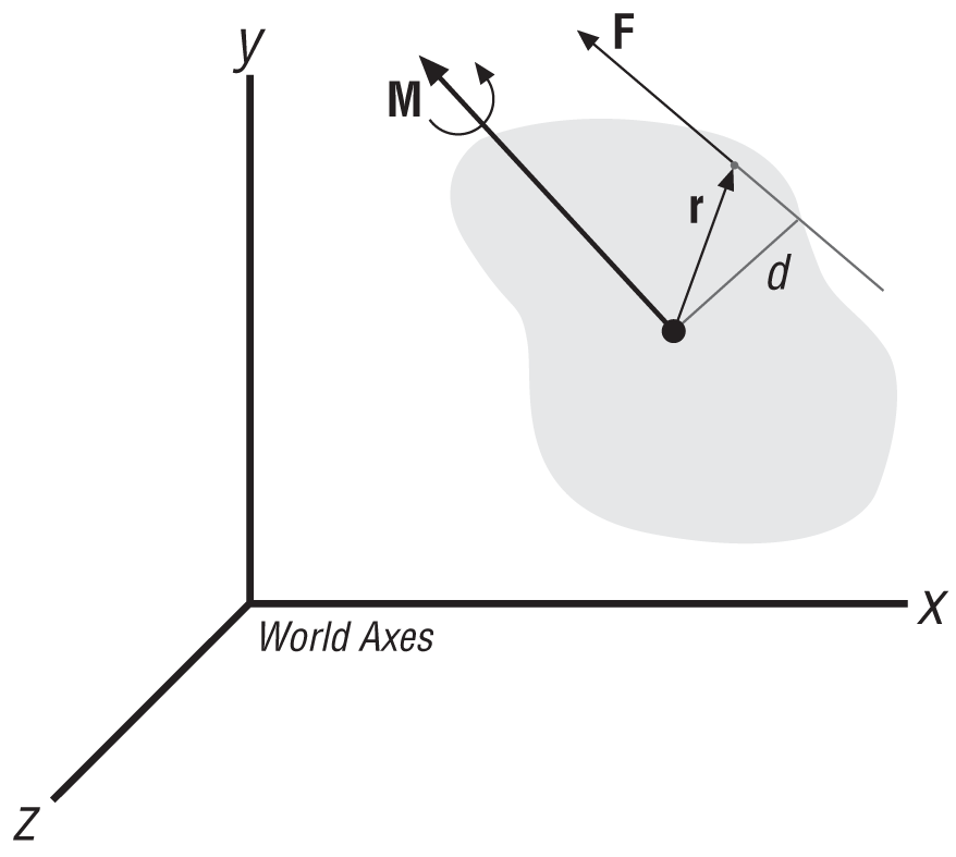
We said earlier that you find the magnitude of torque by multiplying the magnitude of the applied force times the perpendicular distance between the axis of rotation and the line of action of the force. This calculation is easy to perform in two dimensions where the perpendicular distance (d in Figure 3-3) is readily calculable.
However, in three dimensions you’ll want to be able to calculate torque by knowing only the force vector and the coordinates of its point of application on the body relative to the axis of rotation. You can accomplish this by using the following formula:
| M = r × F |
The torque, M, is the vector cross product of the position vector, r, and the force vector, F.
In rectangular coordinates you can write the distance, force, and torque vectors as follows:
| r = x i + y j + z k |
| F = Fx i + Fy j + Fz k |
| M = Mx i + My j + Mz k |
The scalar components of r (x, y, and z) are the coordinate distances from the axis of rotation to the point of application of the force, F. The scalar components of the torque vector, M, are defined by the following:
| Mx = y Fz – z Fy |
| My = z Fx – x Fz |
| Mz = x Fy – y Fx |
Consider the rigid body shown in Figure 3-4 acted upon by the force F at a point away from the body’s center of mass.
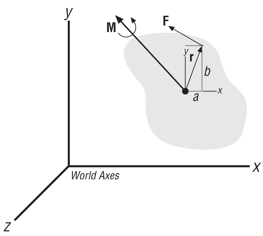
In this example F, a, and b are given and are as follows:
| F = (−90 lbs) i + (156 lbs) j + (0) k |
| a = 0.66 ft |
| b = 0.525 ft |
Calculate the torque about the body’s center of mass due to the force F.
The first step is to put together the distance vector from the point of application of F to the body’s center of mass. Since the local coordinates a and b are given, r is simply:
| r = (0.66 ft) i + (0.525 ft) j + (0) k |
Now using the formula M = r × F (or the formulas for the components of the torque vector shown earlier), you can write:
| M = [(0.66 ft) i + (0.525 ft) j + (0) k] × [(−90 lbs) i + (156 lbs) j + (0) k] |
| M = [(0.66 ft) (156 lbs) – (0.525 ft) (−90 lbs)] k |
| M = (150.2 ft-lbs) k |
Note that the x and y components of the torque vector are 0; thus, the torque moment is pointing directly along the z-axis. The torque vector would be pointing out of the page of this book in this case.
In dynamics you need to consider the sum, or total, of all forces acting on an object separately from the sum of all torques acting on a body. When summing forces, you simply add, vectorally, all of the forces without regard to their point of application. However, when summing torques you must take into account the point of application of the forces to calculate the torques, as shown in the previous example. Then you can take the vector sum of all torques acting on the body.
When you are considering rigid bodies that are not physically constrained to rotate about a fixed axis, any force acting through the body’s center of mass will not produce a torque on the body about its center of gravity. In this case, the axis of rotation passes through the center of mass of the body and the vector r would be 0 (all components 0). When a force acts through a point on the body some distance away from its center of mass, a torque on the body will develop, and the angular motion of the body will be affected. Generally, field forces, which are forces at a distance, are assumed to act through a body’s center of mass; thus, only the body’s linear motion will be affected unless the body is constrained to rotate about a fixed point. Other contact forces, however, generally do not act through a body’s center of mass (they could but aren’t necessarily assumed to) and tend to affect the body’s angular motion as well as its linear motion.
Summary
As we said earlier, this chapter on forces is your bridge from kinematics to kinetics. Here you’ve looked at the major force categories—contact forces and force fields—and some important specific types of forces. This chapter was meant to give you enough theoretical background on forces so you can fully appreciate the subject of kinetics that’s covered in the next chapter. In Chapter 15 through Chapter 19, you’ll revisit the subject of forces from a much more practical point of view when we investigate specific real-life problems. We’ll also introduce some new specific types of force in those chapters that we didn’t cover here.
[9] Static here implies that there is no motion; the block is sitting still with all forces balancing.
[10] The term dynamic is sometimes used here instead of kinetic.
[11] Specific weight is density times the acceleration due to gravity. Typical units are lbs/ft3 and N/m3.
[12] Another common term for torque is moment.