
Chapter 15. Aircraft
If you are going to write a flight simulation game, one of the most important aspects of your game engine will be your flight model. Yes, your 3D graphics, user interface, story, avionics system simulation, and coding are all important, but what really defines the behavior of the aircraft that you are simulating is your flight model. Basically, this is your simplified version of the physics of aircraft flight—that is, your assumptions, approximations, and all the formulas you’ll use to calculate mass, inertia, and lift and drag forces and moments.
There are four major forces that act on an airplane in flight: gravity, lift, thrust, and drag. Gravity, of course, is the force that tends to pull the aircraft to the ground, while lift is the force generated by the wings (or lifting surfaces) of the aircraft to counteract gravity and enable the plane to stay aloft. The thrust force generated by the aircraft’s propulsor (jet engine or propeller) increases the aircraft’s velocity and enables the lifting surfaces to generate lift. Finally, drag counteracts the thrust force, tending to impede the aircraft’s motion. Figure 15-1 illustrates these forces.
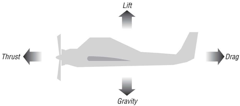
We’ve already discussed the force due to gravity in earlier chapters, so we won’t address it again in this chapter except to say that the total of all lift forces must be greater than or equal to the gravitational force if an aircraft is to maintain flight.
To address the other three forces acting on an aircraft, we’ll refer to a simplified, generic model of an airplane and use it as an illustrative example. There are far too many aircraft types and configurations to treat them all in this short chapter. Moreover, the subject of aerodynamics is too broad and complex. Therefore, the model that we’ll look at will be of a typical subsonic configuration, as shown in Figure 15-2.
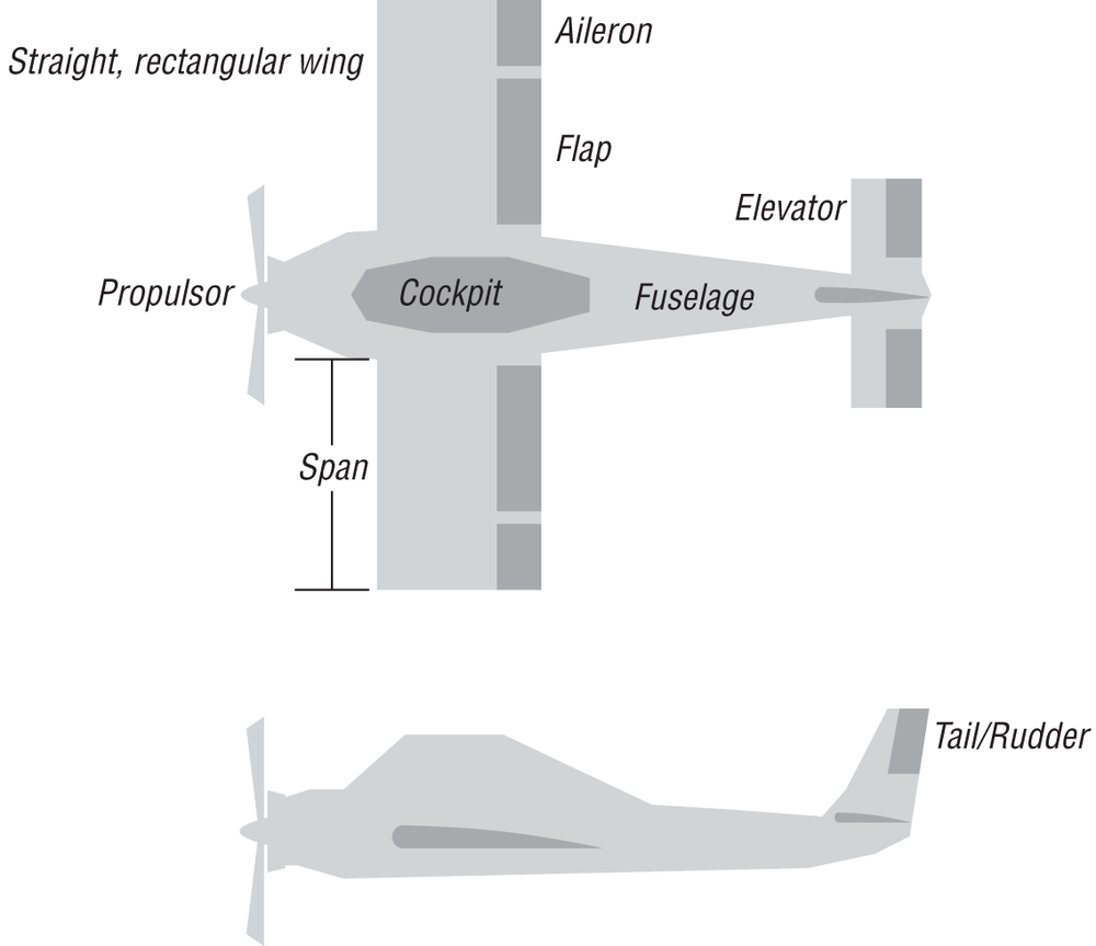
In this configuration the main lifting surfaces (the large wings) are located forward on the aircraft, with relatively smaller lifting surfaces located toward the tail. This is the basic arrangement of most aircraft in existence today.
We’ll have to make some assumptions in order to make even this simplified model manageable. Further, we’ll rely on empirical data and formulas for the calculation of lift and drag forces.
Geometry
Before getting into lift, drag, and thrust, we need to go over some basic geometry and terms to make sure we are speaking the same language. Familiarity with these terms will also help you quickly find what you are looking for when searching through the references that we’ll provide later.
First, take another look at the arrangement of our model aircraft in Figure 15-2. The main body of the aircraft, the part usually occupied by cargo and people, is called the fuselage. The wings are the large rectangular lifting surfaces protruding from the fuselage near the forward end. The longer dimension of the wing is called its span, while its shorter dimension is called its chord length, or simply chord. The ratio of span squared to wing area is called the aspect ratio, and for rectangular wings this reduces to the ratio of span-to-chord.
In our model, the ailerons are located on the outboard ends of the wings. The flaps are also located on the wings inboard of the ailerons. The small wing-like surfaces located near the tail are called elevators. And the vertical flap located on the aft end of the tail is the rudder. We’ll talk more about what these control surfaces do later.
Taking a close look at a cross section of the wing helps to define a few more terms, as shown in Figure 15-3.
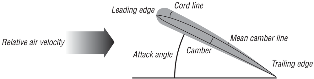
The airfoil shown in Figure 15-3 is a typical cambered airfoil. Camber represents the curvature of the airfoil. If you draw a straight line from the trailing edge to the leading edge, you end up with what’s called the chord line. Now if you divide the airfoil into a number of cross sections, like slices in a loaf of bread, going from the trailing edge to the leading edge, and then draw a curved line passing through the midpoint of each section’s thickness, you end up with the mean camber line. The maximum difference between the mean camber line and the chord line is a measure of the camber of the airfoil. The angle measured between the direction of travel of the airfoil (the relative velocity vector of the airfoil as it passes through the air) and the chord line is called the absolute angle of attack.
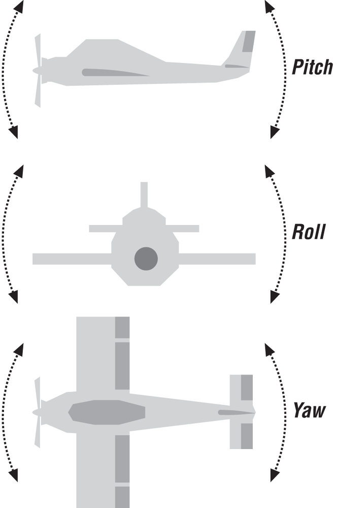
When an aircraft is in flight, it may rotate about any axis. It is standard practice to always refer to an aircraft’s rotations about three axes relative to the pilot. Thus, these axes— the pitch axis, the roll axis, and the yaw axis—are fixed to the aircraft, so to speak, irrespective of its actual orientation in three-dimensional space.
The pitch axis runs transversely across the aircraft—that is, in the port-starboard direction.[23] Pitch rotation is when the nose of the aircraft is raised or lowered from the pilot’s perspective. The roll axis runs longitudinally through the center of the aircraft. Roll motions (rotations) about this axis result in the wing tips being raised or lowered on either side of the pilot. Finally, the yaw axis is a vertical axis about which the nose of the aircraft rotates in the left-to-right (or right-to-left) direction with respect to the pilot. These rotations are illustrated in Figure 15-4.
Lift and Drag
When an airfoil moves through a fluid such as air, lift is produced. The mechanisms by which this occurs are similar to those in the case of the Magnus lift force, discussed earlier in Chapter 6, in that Bernoulli’s law is still in effect. However, this time, instead of rotation it’s the airfoil’s shape and angle of attack that affect the flow of air so as to create lift.
Figure 15-5 shows an airfoil section moving through air at a speed V. V is the relative velocity between the foil and the undisturbed air ahead of the foil. As the air hits and moves around the foil, it splits at the forward stagnation point located near the foil leading edge such that air flows both over and under the foil. The air that flows under the foil gets deflected downward, while the air that flows over the foil speeds up as it goes around the leading edge and over the surface of the foil. The air then flows smoothly off the trailing edge; this is the so-called Kutta condition. Ideally, the boundary layer remains “attached” to the foil without separating as in the case of the sphere discussed in Chapter 6.
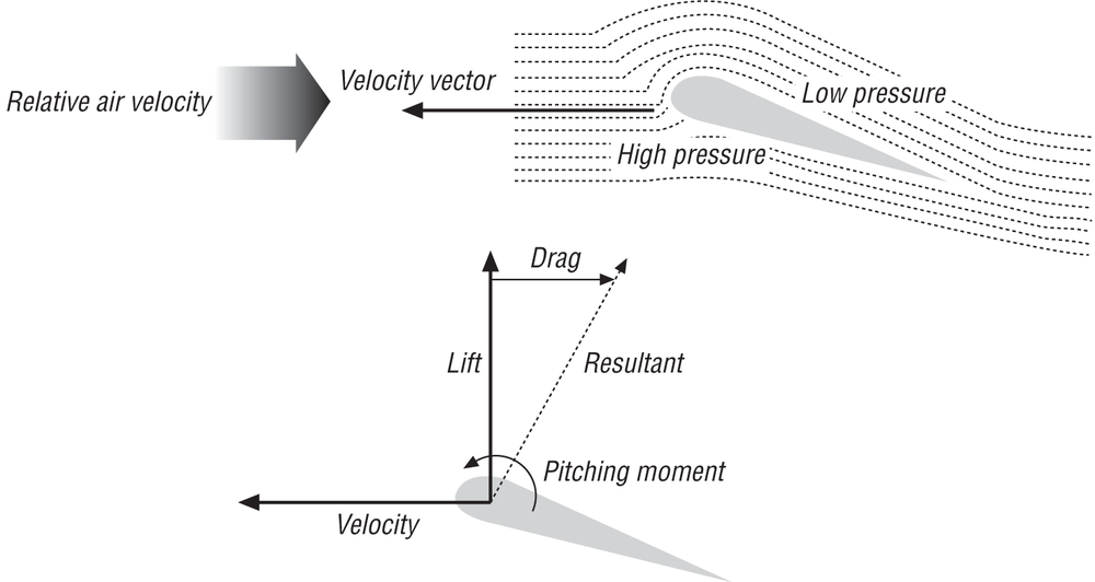
The relatively fast-moving air above the foil results in a region of low pressure above the foil (remember Bernoulli’s equation that shows pressure is inversely proportional to velocity in fluid flow). The air hitting and moving along the underside of the foil creates a region of relatively high pressure. The combined effect of this flow pattern is to create regions of relatively low and high pressure above and below the airfoil. It’s this pressure differential that gives rise to the lift force. By definition, the lift force is perpendicular to the line of flight—that is, the velocity vector.
Note that the airfoil does not have to be cambered in order to generate lift; a flat plate oriented at an angle of attack relative to the airflow will also generate lift. Likewise, an airfoil does not have to have an angle of attack either. Cambered airfoils can generate lift at 0, or even negative, angles of attack. Thus, in general, the total lift force on an airfoil is composed of two components: the lift due to camber and the lift due to attack angle.
Theoretically, the thickness of an airfoil does not contribute to lift. You can, after all, have a thin curved wing as in the case of wings made from fabric (such as those used for hang gliders). In practice, thickness is utilized for structural reasons. Further, thickness at the leading edge can help delay stall (more on this in a moment).
The pressure differential between the upper and lower surfaces of the airfoil also gives rise to a drag force that acts in line with, but opposing, the velocity vector. The lift and drag forces are perpendicular to each other and lie in the plane defined by the velocity vector and the vector normal (perpendicular) to the airfoil chord line. When combined, these two force components, lift and drag, yield the resultant force acting on the airfoil in flight. This is illustrated in Figure 15-5.
Both lift and drag are functions of air density, speed, viscosity, surface area, aspect ratio, and angle of attack. Traditionally, the lift and drag properties of a given foil design are expressed in terms of nondimensional coefficients CL and CD, respectively:
| CL = L / [(1/2) ρ V2 S] |
| CD = D / [(1/2) ρ V2 S] |
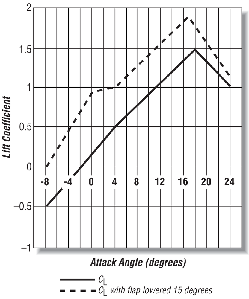
where S is the wing planform area (span times chord for rectangular wings), L is the lift force, D is the drag force, V is the speed through the air, and ρ (rho) is air density. These coefficients are experimentally determined from wind tunnel tests of model airfoil designs at various angles of attack. The results of these tests are usually presented as graphs of lift and drag coefficient versus attack angle. Figure 15-6 through Figure 15-8 illustrate some typical lift and drag charts for a wing section.
The most widely known family of foil section designs and test data is the NACA foil sections. Theory of Wing Sections by Ira H. Abbott and Albert E. Von Doenhoff (Dover) contains a wealth of lift and drag data for practical airfoil designs (see the Bibliography for a complete reference to this work).[24]
In practice, the flow of air around a wing is not strictly two-dimensional—that is, flowing uniformly over each parallel cross section of the wing—and there exists a span-wise flow of air along the wing. The flow is said to be three-dimensional. The more three-dimensional the flow, the less efficient the wing.[25] This effect is reduced on longer, high-aspect-ratio wings (and wings with end plates where the effective aspect ratio is increased); thus, high-aspect-ratio wings are comparatively more efficient.
To account for the effect of aspect ratio, wing sections of various aspect ratios for a given foil design are usually tested so as to produce a family of lift and drag curves versus attack angle. There are other geometrical factors that affect the flow around wings; for a rigorous treatment of these, we refer you to the Theory of Wing Sections and Fluid-Dynamic Lift.[26]
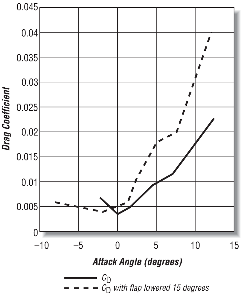
Turning back to Figure 15-6, you’ll notice that the drag coefficient increases sharply with attack angle. This is reasonable, as you would expect the wing to produce the most drag when oriented flat against or perpendicular to the flow of air.
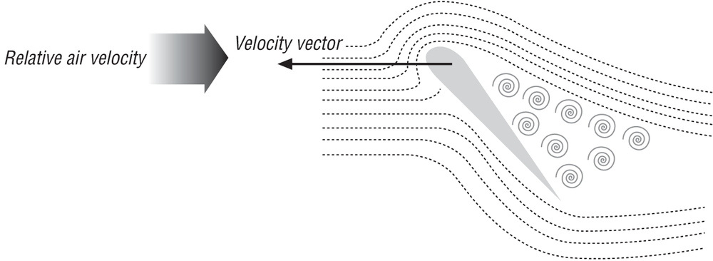
A look at the lift coefficient curve, which initially increases linearly with attack angle, shows that at some attack angle the lift coefficient reaches a maximum value. This angle is called the critical attack angle. For angles beyond the critical, the lift coefficient drops off rapidly and the airfoil (or wing) will stall and cease to produce lift. This is bad. When an aircraft stalls in the air, it will begin to drop rapidly until the pilot corrects the stall situation by, for example, reducing pitch and increasing thrust. When stall occurs, the air no longer flows smoothly over the trailing edge, and the corresponding high angle of attack results in flow separation (as illustrated in Figure 15-9). This loss in lift is also accompanied by an increase in drag.
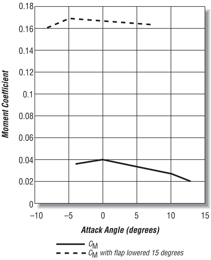
Theoretically, the resultant force acting on an airfoil acts through a point located at one-quarter the chord length aft of the leading edge. This is called the quarter-chord point. In reality, the resultant force line of action will vary depending on attack angle, pressure distribution, and speed, among other factors. However, in practice it is reasonable to assume that the line of action passes through the quarter-chord point for typical operational conditions. To account for the difference between the actual line of action of the resultant and the quarter-chord point, we must consider the pitching moment about the quarter-chord point. This pitching moment tends to tilt the leading edge of the foil down. In some cases this moment is relatively small compared to the other moments acting on the aircraft, and it may be neglected.[27] An exception may be when the foil has deflected flaps.
Flaps are control devices used to alter the shape of the foil so as to change its lift characteristics. Figure 15-6 also shows typical lift, drag, and moment coefficients for an airfoil fitted with a plain flap deflected downward at 15°.[28] Notice the significant increase in lift, drag, and pitch moment when the flap is deflected. Theory of Wing Sections also provides data for flapped airfoils for flap angles between −15° and 60°.
Other Forces
The most notable force that we’ve yet to discuss is thrust—the propulsion force. Thrust provides forward motion; without it, the aircraft’s wings can’t generate lift and the aircraft won’t fly. Thrust, whether generated by a propeller or a jet engine, is usually expressed in pounds, and a common ratio used to compare the relative merits of aircraft powering is the thrust-to-weight ratio. This ratio is the maximum thrust deliverable by the propulsion plant divided by the aircraft’s total weight. When the thrust-to-weight ratio is greater than one, the aircraft is capable of overcoming gravity in a vertical climb. This is more like a rocket than a traditional airplane. Most normal planes are not capable of this, but many military planes do have thrust-to-weight ratios of greater than one. However, airplane engines rely on oxygen in the atmosphere to combust their fuel with and to produce the force that propels them forward. As the plane climbs higher, the engines will have less oxygen and produce less thrust. The thrust-to-weight ratio will fall, and eventually the plane will again need lift from the wings to maintain its altitude. Even when the plane is climbing vertically like a rocket, the wings still generate lift, and in this case try to pull the airplane away from a vertical trajectory.
Besides gravity, thrust, wing lift, and wing drag, there are other forces that act on an aircraft in flight. These are drag forces (and lift in some cases) on the various components of the aircraft besides the wings. For example, the fuselage contributes to the overall drag acting on the aircraft. Additionally, anything sticking out of the fuselage will contribute to the overall drag. If it’s not a wing, anything sticking out of the fuselage is typically called an appendage. Some examples of appendages are the aircraft landing gear, canopy, bombs, missiles, fuel pods, and air intakes.
Typically, drag data for fuselages and appendages is expressed in terms of a drag coefficient similar to that discussed in Chapter 6, where experimentally determined drag forces are nondimensionalized by projected frontal area (S), density (ρ), and velocity squared (V2). This means that the experimentally measured drag force is divided by the quantity (1/2) ρ V2 S to get the dimensionless drag coefficient. Depending on the object under consideration, the drag coefficient data will be presented as a function of some important geometric parameter, such as attack angle in the case of airfoils, or length-to-height ratio in the case of canopies. Here again, Hoerner’s Fluid-Dynamic Drag is an excellent source of practical data for all sorts of fuselage shapes and appendages.
For example, when an aircraft’s landing gear is down, the wheels (as well as associated mechanical gear) contribute to the overall drag force on the aircraft. Hoerner reports drag coefficients based on the frontal area of some small-plane landing-gear designs to be in the range of 0.25 to 0.55. By comparison, drag coefficients for typical external storage pods (such as for fuel), which are usually streamlined, can range from 0.06 to 0.26.
Another component of the total drag force acting on aircraft in flight is due to skin friction. Aircraft wings, fuselages, and appendages are not completely smooth. Weld seams, rivets, and even paint cause surface imperfections that increase frictional drag. As in the case of the sphere data presented in Chapter 6. This frictional drag is dependent on the nature of the flow around the part of the aircraft under consideration—that is, whether the flow is laminar or turbulent. This implies that frictional drag coefficients for specific surfaces will generally be a function of the Reynolds number.
In a rigorous analysis of a specific aircraft’s flight, you’d of course want to consider all these additional drag components. If you’re interested in seeing the nitty-gritty details of such calculations, we suggest you take a look at Chapter 14 of Fluid-Dynamic Drag, where Hoerner gives a detailed example calculation of the total drag force on a fighter aircraft.
Control
The flaps located on the inboard trailing edge of the wing in our model are used to alter the chord and camber of the wing section to increase lift at a given speed. Flaps are used primarily to increase lift during slow speed flight, such as when taking off or landing. When landing, flaps are typically deployed at a high downward angle (downward flap deflections are considered positive) on the order to 30° to 60°. This increases both the lift and drag of the wings. During landing, this increase in drag also assists in slowing the aircraft to a suitable landing speed. During takeoff, this increase in drag works against you in that it necessitates higher thrust to get up to speed; thus, flaps may not be deployed to as great an angle as when you are landing.
Ailerons control or induce roll motion by producing differential lift between the port and starboard wing sections. The basic aileron is nothing more than a pair of trailing-edge flaps fitted to the tips of the wings. These flaps move opposite each other, one deflecting upward and the other downward, to create a lift differential between the port and starboard wings. This lift differential, separated by the distance between the ailerons, creates a torque that rolls the aircraft. To roll the aircraft to the port side (the pilot’s left), the starboard aileron would be deflected in a downward direction while the port aileron would be deflected in an upward direction relative to the pilot. Likewise, the opposite deflections of the ailerons would induce a roll to the starboard side. In a real aircraft, the pilot controls the ailerons by moving the flight stick to either the left or right.
Elevators, the tail “wings,” are used to control the pitch of the aircraft. (Elevators can be flaps, as shown in Figure 15-2, or the entire tail wing can rotate as on the Lockheed Martin F-16.) When the elevators are deflected such that their trailing edge goes down with respect to the pilot, a nose-down pitch rotation will be induced; that is, the tail of the aircraft will tend to rise relative to its nose, and the aircraft will dive. In an actual aircraft, the pilot achieves this by pushing the flight stick forward. When elevators are deflected such that their tailing edge goes up, a nose-up pitch rotation will be induced.
Elevators are very important for trimming (adjusting the pitch of) the aircraft. Generally, the aircraft’s center of gravity is located above the mean quarter-chord line of the aircraft wings such that the center of gravity is in line with the main lift force. However, as we explained earlier, the lift force does not always pass through the quarter-chord point. Further, the aircraft’s center of gravity may very well change during flight—for example, as fuel is burned off and when ordnance is released. By controlling the elevators, the pilot is able to adjust the attitude of the aircraft such that all of the forces balance and the aircraft flies at the desired orientation (pitch angle).
Finally, the rudder is used to control yaw. The pilot uses foot pedals to control the rudder; pushing the left (port) pedal yaws left and pushing the right pedals yaws right (starboard). The rudder is useful for fine-tuning the alignment of the aircraft for approach on landing or when sighting up a target. Typically, large rudder action tends to also induce roll motion that must be compensated for by proper use of the ailerons.
In some cases the rudder consists of a flap on the trailing edge of the vertical tail, while in other cases there is no rudder flap and the entire vertical tail rotates. In both cases, the vertical tail, which also provides directional stability, will usually have a symmetric airfoil shape; that is, its mean camber line will be coincident with its chord line. When the aircraft is flying straight and level, the tail will not generate lift since it is symmetric and its attack angle will be 0. However, if the plane sideslips (yaws relative to its flight direction), then the tail will be at an angle of attack and will generate lift, tending to push the plane back to its original orientation.
Modeling
Although we’ve yet to cover a lot of the material required to implement a real-time flight simulator, we’d like to go ahead and outline some of the steps necessary to calculate the lift and drag forces on your model aircraft:
Discretize the lifting surfaces into a number of smaller wing sections.
Collect geometric and foil performance data.
Calculate the relative air velocity over each wing section.
Calculate the attack angle for each wing section.
Determine the appropriate lift and drag coefficients and calculate lift and drag forces.
The first step is relatively straightforward in that you need to divide the aircraft into smaller sections where each section is approximately uniform in characteristics. Performing this step for the model shown in Figure 15-2, you might divide the wing into four sections—one for each wing section that’s fitted with an aileron and one for each section that’s fitted with a flap. You could also use two sections to model the elevators, one port and one starboard, and another section to model the tail/rudder. Finally, you could lump the entire fuselage together as one additional section or further subdivide it into smaller sections depending on how detailed you want to get.
If you’re going to model your aircraft as a rigid body, you’ll have to account for all of the forces and moments acting on the aircraft while it is in flight. Since the aircraft is composed of a number of different components, each contributing to the total lift and drag, you’ll have to break up your calculations into a number of smaller chunks and then sum all contributions to get the resultant lift and drag forces. You can then use these resultant forces along with thrust and gravity in the equations of motion for your aircraft. You can, of course, refine your model further by adding more components for such items as the cockpit canopy, landing gear, external fuel pods, bombs, etc. The level of detail to which you go depends on the degree of accuracy you’re going for. If you are trying to mimic the flight performance of a specific aircraft, then you need to sharpen your pencil.
Once you’ve defined each section, you must now prepare the appropriate geometric and performance data. For example, for the wings and other lifting surfaces you’ll need to determine each section’s initial incidence angle (its fixed pitch or attack angle relative to the aircraft reference system), span, chord length, aspect ratio, planform area, and quarter-chord location relative to the aircraft’s center of gravity. You’ll also have to prepare a table of lift and drag coefficients versus attack angle appropriate for the section under consideration. Since this data is usually presented in graphical form, you’ll have to pull data from the charts to build your lookup table for use in your game. Finally, you’ll need to calculate the unit normal vector perpendicular to the plane of each wing section. (You’ll need this later when calculating angle of attack.)
These first two steps need only be performed once at the beginning of your game or simulation since the data will remain constant (unless your plane changes shape or its center of gravity shifts during your simulation).
The third step involves calculating the relative velocity between the air and each component so you can calculate lift and drag forces. At first glance, this might seem trivial since the aircraft will be traveling at an air speed that will be known to you during your simulation. However, you must also remember that the aircraft is a rigid body and in addition to the linear velocity of its center of gravity, you must account for its rotational velocity.
Back in Chapter 2, we gave you a formula to calculate the relative velocity of any point on a rigid body that was undergoing both linear and rotational motion:
| vR = vcg + (ω × r) |
This is the formula you’ll need to calculate the relative velocity at each component in your model. In this case, vcg is the vector representing the air speed and flight direction of the aircraft, ω (omega) is the angular velocity vector of the aircraft, and r is the distance vector from the aircraft’s center of gravity to the component under consideration.
When dealing with wings, once you have the relative velocity vector, you can proceed to calculate the attack angle for each wing section. The drag force vector will be parallel to the relative velocity vector, while the lift force vector will be perpendicular to the velocity vector. Angle of attack is then the angle between the lift force vector and the normal vector perpendicular to the plane of the wing section. This involves taking the dot product of these two vectors.
Once you have the attack angle, you can go to your coefficient of lift and drag versus attack angle tables to determine the lift and drag coefficients to use at this instant in your simulation. With these coefficients, you can use the following formulas to estimate the magnitudes of lift and drag forces on the wing section under consideration:
| Lift = CL (1/2) ρ V2 S |
| Drag = CD (1/2) ρ V2 S |
This is a very simplified approach that only approximates the lift and drag characteristics. This approach does not account for span-wise flow effects, or the flow effects between adjacent wing sections. Nor does this approach account for air disturbances, such as downwash, that may affect the relative angle of attack for a wing section. Further, the airflow over each wing section is assumed to be steady and uniform.
As a simple example, consider wing panel 1, which is the starboard aileron wing section. Assume that the wing is set at an initial incidence angle of 3.5° and that the plane is traveling at a speed of 38.58 m/s in level flight at low altitude with a pitch angle of 4.5°. This wing section has a chord length of 1.585 m and the span of this section is 1.829 m. Using the lift and drag data presented in Figure 15-6, calculate the lift and drag on this wing section, assuming the ailerons are not deflected and that the density of air is 1.221 kg/m3.
The first step is to calculate the angle of attack, which is 8°, based on the information provided. Now, looking at Figure 15-6, you can find the airfoil lift and drag coefficients to be 0.92 and 0.013, respectively.
Next, you’ll need to calculate the planform area of this section, which is simply its chord times its span. This yields 2.899 m2. Now you have enough information to calculate lift and drag as follows:
| Lift = CL (1/2) ρ V2 S |
| Lift = 0.92 (1/2) (1.221 kg/m3) (38.58 m/s)2 (2.899 m2) |
| Lift = 2,412.8 N |
| Drag = CD (1/2) ρ V2 S |
| Drag = 0.013 (1/2) (1.221 kg/m3) (38.58 m/s)2 (2.899 m2) |
| Drag = 35.6 N |
In your simulation, you’ll have to perform a similar set of calculations for every component that you’ve defined. As you can see, using this sort of empirical data and formulas, although only approximate, lends itself to fairly easy calculations. The hard part is deciding what to model and finding the right data, and after that the lift and drag calculations are pretty simple.
We’ve prepared an example program to show you how to model a simple airplane using the method shown here. The program is named FlightSim.exe and is a real-time, 3D flight simulator. The small aircraft simulated resembles that shown in Figure 15-2.
This program includes the following source files along with a text file (Instructions.txt) that explains the flight controls:
Physics.cpp and Physics.h
D3dstuff.cpp and D3dstuff.h
Mymath.h
Winmain.cpp
As we said, this program is a real-time simulation, and it treats the aircraft as a rigid body. We’ve covered real-time simulations earlier in this book, and Chapter 12 in particular covered some aspects of this flight simulation; therefore, some of the code to follow will be familiar to you. In this present chapter, though, we’re going to focus on a few specific functions that implement the flight model. These functions are contained in the source file Physics.cpp.
The first function we want you to look at is CalcAirplaneMassProperties:
//------------------------------------------------------------------------//
// This model uses a set of eight discrete elements to represent the
// airplane.  The elements are described below:
//
//          Element 0:  Outboard; port (left) wing section fitted with ailerons
//          Element 1:  Inboard; port wing section fitted with landing flaps
//          Element 2:  Inboard; starboard (right) wing section fitted with
                        landing flaps
//          Element 3:  Outboard; starboard wing section fitted with ailerons
//          Element 4:  Port elevator fitted with flap
//          Element 5:  Starboard elevator fitted with flap
//          Element 6:  Vertical tail/rudder (no flap; the whole thing rotates)
//          Element 7:  The fuselage
//
//  This function first sets up each element and then goes on to calculate
//  the combined weight, center of gravity, and inertia tensor for the plane.
//  Some other properties of each element are also calculated, which you'll
//  need when calculating the lift and drag forces on the plane.
//------------------------------------------------------------------------//
void     CalcAirplaneMassProperties(void)
{
     float     mass;
     Vector    vMoment;
     Vector    CG;
     int       i;
     float     Ixx, Iyy, Izz, Ixy, Ixz, Iyz;
     float     in, di;

     // Initialize the elements here
     // Initially the coordinates of each element are referenced from
     // a design coordinates system located at the very tail end of the plane,
     // its baseline and center line.  Later, these coordinates will be adjusted
     // so that each element is referenced to the combined center of gravity of
     // the airplane.
     Element[0].fMass = 6.56f;
     Element[0].vDCoords = Vector(14.5f,12.0f,2.5f);
     Element[0].vLocalInertia = Vector(13.92f,10.50f,24.00f);
     Element[0].fIncidence = −3.5f;
     Element[0].fDihedral = 0.0f;
     Element[0].fArea = 31.2f;
     Element[0].iFlap = 0;

     Element[1].fMass = 7.31f;
     Element[1].vDCoords = Vector(14.5f,5.5f,2.5f);
     Element[1].vLocalInertia = Vector(21.95f,12.22f,33.67f);
     Element[1].fIncidence = −3.5f;
     Element[1].fDihedral = 0.0f;
     Element[1].fArea = 36.4f;
     Element[1].iFlap = 0;

     Element[2].fMass = 7.31f;
     Element[2].vDCoords = Vector(14.5f,−5.5f,2.5f);
     Element[2].vLocalInertia = Vector(21.95f,12.22f,33.67f);
     Element[2].fIncidence = −3.5f;
     Element[2].fDihedral = 0.0f;
     Element[2].fArea = 36.4f;
     Element[2].iFlap = 0;

     Element[3].fMass = 6.56f;
     Element[3].vDCoords = Vector(14.5f,−12.0f,2.5f);
     Element[3].vLocalInertia = Vector(13.92f,10.50f,24.00f);
     Element[3].fIncidence = −3.5f;
     Element[3].fDihedral = 0.0f;
     Element[3].fArea = 31.2f;
     Element[3].iFlap = 0;

     Element[4].fMass = 2.62f;
     Element[4].vDCoords = Vector(3.03f,2.5f,3.0f);
     Element[4].vLocalInertia = Vector(0.837f,0.385f,1.206f);
     Element[4].fIncidence = 0.0f;
     Element[4].fDihedral = 0.0f;
     Element[4].fArea = 10.8f;
     Element[4].iFlap = 0;

     Element[5].fMass = 2.62f;
     Element[5].vDCoords = Vector(3.03f,−2.5f,3.0f);
     Element[5].vLocalInertia = Vector(0.837f,0.385f,1.206f);
     Element[5].fIncidence = 0.0f;
     Element[5].fDihedral = 0.0f;
     Element[5].fArea = 10.8f;
     Element[5].iFlap = 0;

     Element[6].fMass = 2.93f;
     Element[6].vDCoords = Vector(2.25f,0.0f,5.0f);
     Element[6].vLocalInertia = Vector(1.262f,1.942f,0.718f);
     Element[6].fIncidence = 0.0f;
     Element[6].fDihedral = 90.0f;
     Element[6].fArea = 12.0f;
     Element[6].iFlap = 0;

     Element[7].fMass = 31.8f;
     Element[7].vDCoords = Vector(15.25f,0.0f,1.5f);
     Element[7].vLocalInertia = Vector(66.30f,861.9f,861.9f);
     Element[7].fIncidence = 0.0f;
     Element[7].fDihedral = 0.0f;
     Element[7].fArea = 84.0f;
     Element[7].iFlap = 0;

     // Calculate the vector normal (perpendicular) to each lifting surface.
     // This is required when you are calculating the relative air velocity for
     // lift and drag calculations.
     for (i = 0; i< 8; i++)
     {
          in = DegreesToRadians(Element[i].fIncidence);
          di = DegreesToRadians(Element[i].fDihedral);
          Element[i].vNormal = Vector((float)sin(in), (float)(cos(in)*sin(di)),
                                      (float)(cos(in)*cos(di)));
          Element[i].vNormal.Normalize();
     }

     // Calculate total mass
     mass = 0;
     for (i = 0; i< 8; i++)
          mass += Element[i].fMass;

     // Calculate combined center of gravity location
     vMoment = Vector(0.0f, 0.0f, 0.0f);
     for (i = 0; i< 8; i++)
     {
          vMoment += Element[i].fMass*Element[i].vDCoords;
     }
     CG = vMoment/mass;

     // Calculate coordinates of each element with respect to the combined CG
     for (i = 0; i< 8; i++)
     {
          Element[i].vCGCoords = Element[i].vDCoords − CG;
     }

     // Now calculate the moments and products of inertia for the
     // combined elements.
     // (This inertia matrix (tensor) is in body coordinates)
     Ixx = 0;     Iyy = 0;     Izz = 0;
     Ixy = 0;     Ixz = 0;     Iyz = 0;
     for (i = 0; i< 8; i++)
     {
          Ixx += Element[i].vLocalInertia.x + Element[i].fMass *
                 (Element[i].vCGCoords.y*Element[i].vCGCoords.y +
                 Element[i].vCGCoords.z*Element[i].vCGCoords.z);
          Iyy += Element[i].vLocalInertia.y + Element[i].fMass *
                 (Element[i].vCGCoords.z*Element[i].vCGCoords.z +
                 Element[i].vCGCoords.x*Element[i].vCGCoords.x);
          Izz += Element[i].vLocalInertia.z + Element[i].fMass *
                 (Element[i].vCGCoords.x*Element[i].vCGCoords.x +
                 Element[i].vCGCoords.y*Element[i].vCGCoords.y);
          Ixy += Element[i].fMass * (Element[i].vCGCoords.x *
                 Element[i].vCGCoords.y);
          Ixz += Element[i].fMass * (Element[i].vCGCoords.x *
                 Element[i].vCGCoords.z);
          Iyz += Element[i].fMass * (Element[i].vCGCoords.y *
                 Element[i].vCGCoords.z);
     }

     // Finally, set up the airplane's mass and its inertia matrix and take the
     // inverse of the inertia matrix.
     Airplane.fMass = mass;
     Airplane.mInertia.e11 = Ixx;
     Airplane.mInertia.e12 = -Ixy;
     Airplane.mInertia.e13 = -Ixz;
     Airplane.mInertia.e21 = -Ixy;
     Airplane.mInertia.e22 = Iyy;
     Airplane.mInertia.e23 = -Iyz;
     Airplane.mInertia.e31 = -Ixz;
     Airplane.mInertia.e32 = -Iyz;
     Airplane.mInertia.e33 = Izz;

     Airplane.mInertiaInverse = Airplane.mInertia.Inverse();
}
Among other things, this function essentially completes step 1 (and part of step 2) of our modeling method: discretize the airplane into a number of smaller pieces, each with its own mass and lift and drag properties. For this model we chose to use eight pieces, or elements, to describe the aircraft. Our comments at the beginning of the function explain what each element represents.
The very first thing this function does is initialize the elements with the properties that we’ve defined to approximate the aircraft. Each element is given a mass, a set of design coordinates to its center of mass, a set of moments of inertia about each element’s center of mass, an initial incidence angle, a planform area, and a dihedral angle.
The design coordinates are the coordinates of the element with respect to an origin located at the very tip of the aircraft’s tail, on its centerline and at its baseline. The x-axis of this system points toward the nose of the aircraft, while the y-axis points toward the port side. The z-axis points up. You have to set up your elements in this design coordinate system first because you don’t yet know the location of the whole aircraft’s center of mass, which is the combined center of mass of all of the elements. Ultimately, you want each element referenced from the combined center of mass because it’s the center of mass that you’ll track during the simulation.
The dihedral angle is the angle about the x-axis at which the element is initially set. For our model, all of the elements have a 0 dihedral angle; that is, they are horizontal, except for the tail rudder, which has a 90° dihedral since it is oriented vertically.
After we’ve set up the elements, the first calculation that this function performs is to find the unit normal vector to each element’s surface based on the element’s incidence and dihedral angles. You need this direction vector to help calculate the angle of attack between the airflow and the element.
The next calculation is the total mass calculation, which is simply the sum of all element masses. Immediately following that, we determine the combined center of gravity location using the technique we discussed in Chapter 1. The coordinates to the combined center of gravity are referenced to the design coordinate system. You need to subtract this coordinate from the design coordinate of each element in order to determine each element’s coordinates relative to the combined center of gravity. After that, you’re all set with the exception of the combined moment of inertia tensor, which we already discussed in Chapter 11 and Chapter 12.
Step 2 of our modeling method says you need to collect the airfoil performance data. For the example program, we used a cambered airfoil with plain flaps to model the wings and elevators, and we used a symmetric airfoil without flaps to model the tail rudder. We didn’t use flaps for the tail rudder since we just made the whole thing rotate about a vertical axis to provide rudder action.
For the wings, we set up two functions to handle the lift and drag coefficients:
//------------------------------------------------------------------------//
//  Given the attack angle and the status of the flaps, this function
//  returns the appropriate lift coefficient for a cambered airfoil with
//  a plain trailing-edge flap (+/- 15 degree deflection).
//------------------------------------------------------------------------//
float     LiftCoefficient(float angle, int flaps)
{
     float clf0[9] = {−0.54f, −0.2f, 0.2f, 0.57f, 0.92f, 1.21f, 1.43f, 1.4f,
                      1.0f};
     float clfd[9] = {0.0f, 0.45f, 0.85f, 1.02f, 1.39f, 1.65f, 1.75f, 1.38f,
                      1.17f};
     float clfu[9] = {−0.74f, −0.4f, 0.0f, 0.27f, 0.63f, 0.92f, 1.03f, 1.1f,
                      0.78f};
     float a[9]      = {−8.0f, −4.0f, 0.0f, 4.0f, 8.0f, 12.0f, 16.0f, 20.0f,
                        24.0f};
     float cl;
     int   i;

     cl = 0;
     for (i=0; i<8; i++)
     {
          if( (a[i] <= angle) && (a[i+1] > angle) )
          {
               switch(flaps)
               {
                    case 0:// flaps not deflected
                         cl = clf0[i] - (a[i] - angle) * (clf0[i] - clf0[i+1]) /
                             (a[i] - a[i+1]);
                         break;
                    case −1: // flaps down
                         cl = clfd[i] - (a[i] - angle) * (clfd[i] - clfd[i+1]) /
                             (a[i] - a[i+1]);
                         break;
                    case 1: // flaps up
                         cl = clfu[i] - (a[i] - angle) * (clfu[i] - clfu[i+1]) /
                             (a[i] - a[i+1]);
                         break;
               }
               break;
          }
     }

     return cl;
}

//------------------------------------------------------------------------//
//  Given the attack angle and the status of the flaps, this function
//  returns the appropriate drag coefficient for a cambered airfoil with
//  a plain trailing-edge flap (+/- 15 degree deflection).
//------------------------------------------------------------------------//
float     DragCoefficient(float angle, int flaps)
{
     float cdf0[9] = {0.01f, 0.0074f, 0.004f, 0.009f, 0.013f, 0.023f, 0.05f,
                      0.12f, 0.21f};
     float cdfd[9] = {0.0065f, 0.0043f, 0.0055f, 0.0153f, 0.0221f, 0.0391f, 0.1f,
                      0.195f, 0.3f};
     float cdfu[9] = {0.005f, 0.0043f, 0.0055f, 0.02601f, 0.03757f, 0.06647f,
                      0.13f, 0.18f, 0.25f};
     float a[9]      = {−8.0f, −4.0f, 0.0f, 4.0f, 8.0f, 12.0f, 16.0f, 20.0f,
                        24.0f};
     float cd;
     int   i;

     cd = 0.5;
     for (i=0; i<8; i++)
     {
          if( (a[i] <= angle) && (a[i+1] > angle) )
          {
               switch(flaps)
               {
                    case 0:// flaps not deflected
                         cd = cdf0[i] - (a[i] - angle) * (cdf0[i] - cdf0[i+1]) /
                              (a[i] - a[i+1]);
                         break;
                    case −1: // flaps down
                         cd = cdfd[i] - (a[i] - angle) * (cdfd[i] - cdfd[i+1]) /
                              (a[i] - a[i+1]);
                         break;
                    case 1: // flaps up
                         cd = cdfu[i] - (a[i] - angle) * (cdfu[i] - cdfu[i+1]) /
                              (a[i] - a[i+1]);
                         break;
               }
               break;
          }
     }

     return cd;

}
Each of these functions takes the angle of attack as a parameter along with a flag used to indicate the state of the flaps—that is, whether the flaps are in neutral position, deflected downward, or deflected upward. Notice that the lift and drag coefficient data is given for a set of discrete attack angles, thus we use linear interpolation to determine the coefficients for attack angles that fall between the discrete angles.
The functions for determining the tail rudder lift and drag coefficients are similar to those shown here for the wings, with the only differences being the coefficients themselves and the fact that the tail rudder does not include flaps. Here are the functions:
//------------------------------------------------------------------------//
//  Given the attack angle, this function returns the proper lift coefficient
//  for a symmetric (no camber) airfoil without flaps.
//------------------------------------------------------------------------//
float     RudderLiftCoefficient(float angle)
{
     float clf0[7] = {0.16f, 0.456f, 0.736f, 0.968f, 1.144f, 1.12f, 0.8f};
     float a[7]      = {0.0f, 4.0f, 8.0f, 12.0f, 16.0f, 20.0f, 24.0f};
     float cl;
     int       i;
     float     aa = (float) fabs(angle);

     cl = 0;
     for (i=0; i<8; i++)
     {
          if( (a[i] <= aa) && (a[i+1] > aa) )
          {
               cl = clf0[i] - (a[i] - aa) * (clf0[i] - clf0[i+1]) /
                   (a[i] - a[i+1]);
               if (angle < 0) cl = -cl;
               break;
          }
     }
     return cl;
}

//------------------------------------------------------------------------//
//  Given the attack angle, this function returns the proper drag coefficient
//  for a symmetric (no camber) airfoil without flaps.
//------------------------------------------------------------------------//
float     RudderDragCoefficient(float angle)
{
     float cdf0[7] = {0.0032f, 0.0072f, 0.0104f, 0.0184f, 0.04f, 0.096f, 0.168f};
     float a[7]      = {0.0f, 4.0f, 8.0f, 12.0f, 16.0f, 20.0f, 24.0f};
     float cd;
     int       i;
     float     aa = (float) fabs(angle);

     cd = 0.5;
     for (i=0; i<8; i++)
     {
          if( (a[i] <= aa) && (a[i+1] > aa) )
          {
               cd = cdf0[i] - (a[i] - aa) * (cdf0[i] - cdf0[i+1]) /
                   (a[i] - a[i+1]);
               break;
          }
     }
     return cd;
}
With steps 1 and 2 out of the way, steps 3, 4, and 5 are handled in
a single function called CalcAirplaneLoads:
//------------------------------------------------------------------------//
// This function calculates all of the forces and moments acting on the
// plane at any given time.
//------------------------------------------------------------------------//
void     CalcAirplaneLoads(void)
{
     Vector     Fb, Mb;

     // reset forces and moments:
     Airplane.vForces.x = 0.0f;
     Airplane.vForces.y = 0.0f;
     Airplane.vForces.z = 0.0f;

     Airplane.vMoments.x = 0.0f;
     Airplane.vMoments.y = 0.0f;
     Airplane.vMoments.z = 0.0f;

     Fb.x = 0.0f;     Mb.x = 0.0f;
     Fb.y = 0.0f;     Mb.y = 0.0f;
     Fb.z = 0.0f;     Mb.z = 0.0f;

     // Define the thrust vector, which acts through the plane's CG
     Thrust.x = 1.0f;
     Thrust.y = 0.0f;
     Thrust.z = 0.0f;
     Thrust *= ThrustForce;

     // Calculate forces and moments in body space:
     Vector    vLocalVelocity;
     float     fLocalSpeed;
     Vector    vDragVector;
     Vector    vLiftVector;
     float     fAttackAngle;
     float     tmp;
     Vector    vResultant;
     int       i;
     Vector    vtmp;

     Stalling = false;

     for(i=0; i<7; i++) // loop through the seven lifting elements
                        // skipping the fuselage
     {
          if (i == 6) // The tail/rudder is a special case since it can rotate;
          {           // thus, you have to recalculate the normal vector.
               float in, di;
               in = DegreesToRadians(Element[i].fIncidence); // incidence angle
               di = DegreesToRadians(Element[i].fDihedral);  // dihedral angle
               Element[i].vNormal = Vector(     (float)sin(in),
                                                (float)(cos(in)*sin(di)),
                                                (float)(cos(in)*cos(di)));
               Element[i].vNormal.Normalize();
          }

          // Calculate local velocity at element
          // The local velocity includes the velocity due to linear
          // motion of the airplane,
          // plus the velocity at each element due to the
          // rotation of the airplane.

          // Here's the rotational part
          vtmp = Airplane.vAngularVelocity^Element[i].vCGCoords;

          vLocalVelocity = Airplane.vVelocityBody + vtmp;

          // Calculate local air speed
          fLocalSpeed = vLocalVelocity.Magnitude();

          // Find the direction in which drag will act.
          // Drag always acts inline with the relative
          // velocity but in the opposing direction
          if(fLocalSpeed > 1.)
               vDragVector = -vLocalVelocity/fLocalSpeed;

          // Find the direction in which lift will act.
          // Lift is always perpendicular to the drag vector
          vLiftVector = (vDragVector^Element[i].vNormal)^vDragVector;
          tmp = vLiftVector.Magnitude();
          vLiftVector.Normalize();

          // Find the angle of attack.
          // The attack angle is the angle between the lift vector and the
          // element normal vector. Note, the sine of the attack angle
          // is equal to the cosine of the angle between the drag vector and
          // the normal vector.
          tmp = vDragVector*Element[i].vNormal;
          if(tmp > 1.) tmp = 1;
          if(tmp < −1) tmp = −1;
          fAttackAngle = RadiansToDegrees((float) asin(tmp));

          // Determine the resultant force (lift and drag) on the element.
          tmp = 0.5f * rho * fLocalSpeed*fLocalSpeed * Element[i].fArea;
          if (i == 6) // Tail/rudder
          {
               vResultant =  (vLiftVector*RudderLiftCoefficient(fAttackAngle) +
                              vDragVector*RudderDragCoefficient(fAttackAngle))
                              * tmp;
          } else
               vResultant =  (vLiftVector*LiftCoefficient(fAttackAngle,
                              Element[i].iFlap) +
                              vDragVector*DragCoefficient(fAttackAngle,
                              Element[i].iFlap) ) * tmp;
          // Check for stall.
          // We can easily determine stall by noting when the coefficient
          // of lift is 0. In reality, stall warning devices give warnings well
          // before the lift goes to 0 to give the pilot time to correct.
          if (i<=0)
          {
               if (LiftCoefficient(fAttackAngle, Element[i].iFlap) == 0)
                    Stalling = true;
          }

          // Keep a running total of these resultant forces (total force)
          Fb += vResultant;

          // Calculate the moment about the CG of this element's force
          // and keep a running total of these moments (total moment)
          vtmp = Element[i].vCGCoords^vResultant;
          Mb += vtmp;
     }

     // Now add the thrust
     Fb += Thrust;

     // Convert forces from model space to earth space
     Airplane.vForces = QVRotate(Airplane.qOrientation, Fb);

     // Apply gravity (g is defined as −32.174 ft/s^2)
     Airplane.vForces.z += g * Airplane.fMass;

     Airplane.vMoments += Mb;
}
The first thing this function does is reset the variables that hold the total force and moment acting on the aircraft. Next, the thrust vector is set up. This is trivial in this example since we’re assuming that the thrust vector always points in the plus x-axis direction (toward the nose) and passes through the aircraft center of gravity (so it does not create a moment).
After calculating the thrust vector, the function loops over the model elements to calculate the lift and drag forces on each element. We’ve skipped the fuselage in this model; however, if you want to account for its drag in your model, this is the place to add the drag calculation.
Going into the loop, the first thing the function does is check to see if the current element is element number six, the tail rudder. If it is, then the rudder’s normal vector is recalculated based on the current incidence angle. The incidence angle for the rudder is altered when you press the X or C keys to apply rudder action.
The next calculation is to determine the relative velocity between the air and the element under consideration. As we stated earlier, this relative velocity consists of the linear velocity as the airplane moves through the air plus the velocity of each element due to the airplane’s rotation. Once you’ve obtained this vector, you calculate the relative air speed by taking the magnitude of the relative velocity vector.
The next step is to determine the direction in which drag will act. Since drag opposes motion, it acts inline with, but opposite to, the relative velocity vector; thus, all you need to do is take the negative of the relative velocity vector and normalize the result (divide it by its magnitude) to obtain the drag direction vector. Since this vector was normalized, its length is equal to 1 (unity), so you can multiply it by the drag force that will be calculated later to get the drag force vector.
After obtaining the drag direction vector, this function uses it to determine the lift direction vector. The lift force vector is always perpendicular to the drag force vector, so to calculate its direction you first take the cross product of the drag direction vector with the element normal vector and then cross the result with the drag direction vector again. Here again, the function normalizes the lift direction vector.
Now that the lift and drag direction vectors have been obtained, the function proceeds to calculate the angle of attack for the current element. The attack angle is the angle between the lift vector and the element normal. You can calculate the angle by taking the inverse cosine of the vector dot product of the lift direction vector with the element normal vector. Since the drag vector is perpendicular to the lift vector, you can get the same result by taking the inverse sine of the vector dot product of the drag direction vector with the element normal vector.
Now with all the lift and drag vector stuff out of the way, the function goes on to calculate the resultant force acting on the element. The resultant force vector is simply the vector sum of the lift and drag force vectors. Notice that this is where the lift and drag coefficient functions are called and where the empirical lift and drag formulas previously discussed are applied.
After calculating the resultant force, the function checks to see if the calculated lift coefficient is 0. If it is, then the stall flag is set to warn us that the plane is in a stalled situation.
Finally, the resultant force is accumulated in the total force vector variable, and we calculate the moment by taking the cross product of the element coordinate vector with the resultant force. The resulting moment is accumulated in the total moment vector variable. After exiting the loop, the function adds the thrust vector to the total force.
So far, all of these forces and moments have been referenced in the body-fixed-coordinate system. The only thing left to do now is apply the gravity force, but this force acts in the negative y-axis direction in the earth-fixed-coordinate system. To apply the gravity force, the function must first rotate the body force vector from body space to earth space coordinates. We used a quaternion rotation technique in this example, which we already discussed in Chapter 11 and Chapter 12.
That’s pretty much it for the flight model. We encourage you to play with the flight model in this program. Go ahead and tweak the element properties and watch to see what happens. Even though this is a rough model, the flight results look quite realistic.
[23] Port is to the pilot’s left and starboard is to the pilot’s right when he or she is sitting in the cockpit facing forward.
[24] Theory of Wing Sections includes standard foil section geometry and performance data, including the well-known NACA family of foil sections. The appendixes to Theory of Wing Sections have all the data you need to collect lift and drag coefficient data for various airfoil designs, including those with flaps.
[25] Lifting efficiency can be expressed in terms of lift-to-drag ratio. The higher the lift-to-drag ratio, the more efficient the wing or foil section.
[26] Fluid-Dynamic Lift, by Sighard F. Hoerner and Henry V. Borst, and Fluid-Dynamic Drag, by Sighard F. Hoerner (both self-published by Hoerner), contain tons of practical charts, tables, and formulas for virtually every aspect of aircraft aerodynamics. They even include material appropriate for high-speed boats and automobiles.
[27] Aircraft designers must always consider this pitching moment when designing the aircraft’s structure, as this moment tends to want to twist the wings off the fuselage.
[28] There’s a large variety of flap designs besides the plain trailing-edge flap discussed here. Flaps are typically referred to in the literature as high lift devices, and the references we’ll provide in this chapter give rough descriptions of the most common designs.