29. Probability

“Probability is the bane of the age,” said Moreland, now warming up. “Every Tom, Dick, and Harry thinks he knows what is probable. The fact is most people have not the smallest idea what is going on round them. Their conclusions about life are based on utterly irrelevant—and usually inaccurate—premises.”

—ANTHONY POWELL, A DANCE TO THE MUSIC OF TIME

One of my favorite probability stories comes from Nobel laureate Manfred Eigen’s Laws of the Game.¹ A man is about to take a long plane trip, but he is concerned about all the bomb threats and hijackings he sees on the news. He calls his insurance agent, who tells him that the risk of a bomb being on the plane is very small. Undeterred, the man asks the agent what the odds are of there being two bombs on his plane. The agent, flustered, says that the probability should be astronomically small. If the odds of one bomb were 1 in 10,000, then the odds of two bombs should be 1 in a 100 million. The man seems calmed by this. A few weeks later, the agent sees on the news that a bomb was seized from a local passenger’s suitcase. At trial, the man claims that he only took the bomb onboard to lower the risk of another bomb being onboard.

¹ Eigen, M., & Winkler, R. (1981). Laws of the Game: How the Principles of Nature Govern Chance. New York: Knopf.

A skill that is perhaps one of the most important in order to be a successful game designer is a strong understanding of the concept of probability. From simple card games to sprawling massively multiplayer online (MMO) games, all use probability as core to their game experience. An innate understanding of probability is essential to making wise gut decisions.

Probability Is Counting

The reason probability scares a lot of new designers is that they think it’s math. Something happened in schools across the world to make people get gun-shy about math. Probability calculations can get hairy and complicated, but at its basest level, probability is nothing more than counting.

Probability = Count of Specific Event / Count of All Events

As an example, you want to know how many times a player will be dealt an ace as his hole card in a game of baccarat. There are four aces in a deck of 52 cards. The item you want the probability of is “Drawing an Ace.” All events would be “Drawing a Card.” So here you would have to count the number of aces and the number of unique cards. So the probability of drawing an ace is as follows:

Count of Aces / Count of Number of Unique Cards = 4 / 52 = 7.7%

Joint Probability

The most common probability operation you’ll likely perform is finding a joint probability. Joint probability is the odds of multiple events occurring at the same time. Before I cover the mathematical way of finding joint probability, I’ll start with an easier example that mostly involves counting.

You have three fair coins: a penny, a nickel, and a dime. If you flip all of them, what are the odds that they all land heads? What are the odds that you get exactly two heads? Since there are only three coins, this is easy to count.

These three coins can land in eight different configurations (Figure 29.1). How many of these configurations have all three as heads? Since only one configuration out of eight does and the odds of every coin are fair, the probability of getting all three heads is one in eight. How many have exactly two heads? If you look at the table in Figure 29.1, you see that there are three: HTH, HHT, THH. Therefore the probability of getting exactly two heads is three in eight.

This was just counting, but if you have larger permutations, the counting can get massive. Luckily, there is an easier way.

Figure 29.1 Flipping three fair coins.

First, here are some principles you need to understand:

• Probability will always be a number between 0 and 1 inclusively. A 0 means the event never happens; 1 means the event always happens. Any number larger than 1 does not make sense because how can something happen more than always? Likewise, less than 0 makes no sense. How can something happen less often than never?

• Probability is represented in a number of ways. Sometimes it’s in fractional form. Sometimes it’s in decimal form. Sometimes it’s in percentage form. The value ½ is equivalent to 0.5 is equivalent to 50 percent. These all say the same thing.

• Shorthand for the probability of an event is generally represented by P(Event) where “Event” is some notation for when you want the probability to be counted. So P(Heads) is another way of saying “the probability of flipping heads.”

The probability of all disjoint (mutually exclusive) events adds up to 1. Disjoint means that no occurrence can happen in more than one event. For instance, a person can be 64 years old or 65 years old, but not both. So the event of “being 64” and the event of “being 65” are disjoint. However, “likes pancakes” and “is American” are not disjoint since both can happen simultaneously. When you have disjoint events, you can add up their probability to get the probability of at least one of the events happening. “Is a registered Republican,” “Is a registered Democrat,” and “Is neither a registered Republican nor a registered Democrat” are disjoint events that reflect all Americans who are registered to vote. Therefore if you add up these three probabilities, you are guaranteed to get 1.

What are the odds of flipping the penny and getting heads? There are two faces, each with equal probability, so just by counting, we know that the odds of getting heads is 1 in 2, or ½, or 0.50. The odds of getting heads on the nickel and dime are the same.

When two events are independent—meaning that what happens in the event doesn’t affect the probability of the other event—you can find the joint probability of all those things happening together by multiplying the probabilities together. Another way of explaining joint probability is by thinking of it as ANDs. The probability of all three being heads can be written as follows:

Probability of (Penny being heads AND Nickel being heads AND Dime being heads)

P of (Penny being heads) * P of (Nickel being heads) * P of (Dime being heads)

(1/2) * (1/2) * (1/2) = 1/8

This is a little more complicated for finding out the probability of the three coin flips resulting in exactly two heads. What are all the ways you can get exactly two heads results?

P(Penny=H AND Nickel=H AND Dime=T)

P(Penny=T AND Nickel=H AND Dime=H)

P(Penny=H AND Nickel=T AND Dime=H)

Since these coin flips are independent, you can find the probability by multiplying the probabilities of these coin flips:

P(Penny=H AND Nickel=H AND Dime=T) = (1/2)*(1/2)*(1/2) = 1/8

P(Penny=T AND Nickel=H AND Dime=H) = (1/2)*(1/2)*(1/2) = 1/8

P(Penny=H AND Nickel=T AND Dime=H) = (1/2)*(1/2)*(1/2) = 1/8

P(Getting exactly two heads) = 1/8 + 1/8 + 1/8 = 3/8

This is easy when you are using even (½ and ½) probabilities. However, change the exercise so the coin is a trick coin that is no longer fair and lands heads 70 percent of the time instead of 50 percent of the time. Now, the counting exercise cannot be used because a heads landing does not happen with the same weight as a tails landing. Here you must use the following math:

P(Penny=H AND Nickel=H AND Dime=T) = (0.7)*(0.7)*(0.3) = 0.147

P(Penny=T AND Nickel=H AND Dime=H) = (0.3)*(0.7)*(0.7) = 0.147

P(Penny=H AND Nickel=T AND Dime=H) = (0.7)*(0.3)*(0.3) = 0.147

P(Getting exactly two heads) = 0.147 + 0.147 + 0.147 = 0.441

Go back to the baccarat example of drawing an ace. The probability of drawing an ace is 1⁄13. If the baccarat deck is a standard deck of cards, what are the odds of the next card being an ace as well? Since the odds of getting one ace are 1⁄13, then the odds of getting two aces should be 1⁄13 * 1⁄13 = 1⁄169 or 0.006 or 0.6 percent, right? Not quite.

Remember that you can multiply probabilities only if the events are independent. These events are not independent because once you have drawn the first ace out of the deck, fewer aces are left in the deck to draw. Just by counting, you knew that the odds of the first card being an ace are 4 in 52, or 0.077. If the first card is an ace, then the odds of getting the next card to be an ace as well are 3 in 51, or 0.059 (or 4 aces minus the one already drawn, and 52 cards minus the one already drawn). Drawing that first ace changes the odds from 7.7 percent to 5.9 percent. Thus, the actual probability of drawing two aces is as follows:

P(Drawing two aces) = P(Drawing first ace) * P(Drawing second ace)

P(Drawing two aces) = (4/52) * (3/51)

P(Drawing two aces) = 12/2652 or 0.0045 or 0.45%

Note that this is much less likely than our original estimate of 0.6 percent!

Conditional Probability

When dealing with events that are dependent on others, it can be helpful to use what is called conditional probability. In conditional probability, you use the fact that some other event has occurred to change the probability of another event. As an example, say that you are doing market research for a children’s game and you need to choose between ponies and spaceships for your theme. You do a survey of ten kids to ask them what they prefer (Figure 29.2)

Figure 29.2 The themes the kids want.

To find the probability that a kid would prefer ponies or spaceships is just simple counting:

P(Ponies) = 4/10 or 40%

P(Spaceships) = 6/10 or 60%

Also, our demographics can be found just by counting:

P(Boy) = 7/10 or 70%

P(Girl) = 3/10 or 30%

Now you have to be careful about how you ask your questions. If you have a boy gamer, what is the probability that he will choose spaceships? This is a different question than what is the probability that a gamer is both a boy and chooses spaceships. For the latter, you count the five boys who said “spaceships” and divide by the ten total kids to get 5/10 or 50 percent. You cannot just multiply the 70 percent chance of picking a boy and the 60 percent chance of picking someone who said “spaceships” and multiply them together, because they are not independent.

The former question already assumes that you have a boy gamer, you would not count the three girl gamers. The answer to the former question is 5/7 or 71.4 percent.

The question “what is the probability that a gamer is both a boy and chose spaceships?” is notated like this:

P(Boy and Spaceships)

The question “given a boy, what is the probability that he will choose spaceships?” is notated like this:

P(Spaceships|Boy)

The vertical pipe means “given,” so you read this as “Probability of Spaceships given Boy.”

A helpful formula is this:

P(A and B) = P(B|A) * P(A)

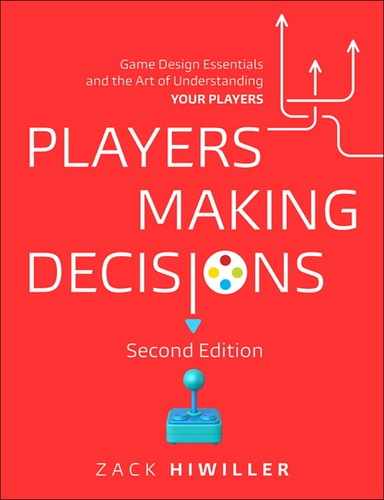
Which is better illustrated by the classic Venn diagram in Figure 29.3.

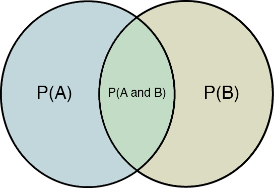
Figure 29.3 Venn diagram.

The value of P(B|A) is represented by the proportion of the P(A) circle that is also P(A and B). This is because you know A is true because you are given A. Therefore, you can ignore all things that are not A. This may be easier to see if you use something countable (remember that overlapping squares count twice, once for A and once for B), as in Figure 29.4.

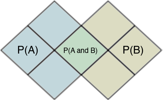
Figure 29.4 Countable Venn diagram.

You have eight total squares. If you know A is true, then you need to look only at the squares that count toward P(A). So when you ask for P(B|A), you look only at those four squares and count the ones that are also counted in P(B). In this case, there are four squares that are “given” as A. So given those four squares, what is the probability of B being in them? There is one square in those four that is also B, so the answer is 1/4.

P(A and B) = P(B|A) * P(A)

(1/8) = (1/4) * (4/8)

Back to the survey:

P(Spaceships | Boy) = P(Boy) / P(Boy and Spaceships)

P(Spaceships | Boy) = (7/10 / (5/10)

P(Spaceships | Boy) = 5/7

Because the example is so simple, you can just count all three quantities, but this is not always the case.

Let’s say you are playing in an online gauntlet match in which the winner stays alive and gains more loot and the loser is knocked out. The probability of any player staying alive for X games or P(X) is as follows:

P(1) = 1.00

P(2) = 0.50

P(3) = 0.24

P(4) = 0.10

P(5) = 0.06

P(6) = 0.02

Let’s say you have successfully won your fourth game. What is the probability that you will win the next game? This is a conditional probability. Given that you have won four, what is the probability that you will win at least five?

P(4 and 5) = P(5|4) / P(4)

But P(4 and 5) = P(5) because if someone has survived their fifth game, then they have survived their fourth by definition. So:

P(5|4) = P(5) / P(4)

P(5|4) = 0.06 / 0.1 = 60%

Not bad odds!

Adding Die Rolls

A common frustration in learning probability can be easily demonstrated by the common mistakes that surround the probability events with multiple die rolls.

To start, what are the odds of rolling a 4 or higher on a six-sided die? This is easily calculated since the events are simple:

P(Getting a 4 or higher) = P(4) + P(5) + P(6)

P(Getting a 4 or higher) = 1/6 + 1/6 + 1/6

P(Getting a 4 or higher) = 3/6 or 0.50 or 50%

To create the stats for a Dungeons & Dragons character, one method is to roll three six-sided dice and add up the results.² Thus, a character’s score can be anywhere from 3 and 18. This is written in shorthand notion to be 3d6 (or three die rolls of six-sided dice). What are the odds of getting a 16 or higher?

² Cook, D. (1989). Advanced Dungeons & Dragons, 2nd Edition, Player’s Handbook. Lake Geneva, Wisconsin: TSR.

The naive way to calculate this is to say that there are 16 possible outcomes that are disjoint between getting a 3 and getting an 18, and three of those (16, 17, 18) are 16 or higher, so the odds must be 3/16.

P(Getting a 16 or higher) = P(16) + P(17) + P(18)

P(Getting a 16 or higher) = 1/16 + 1/16 + 1/16

P(Getting a 16 or higher) = 3/16 or 0.1875 or 18.75%

This is, unfortunately, incorrect. It assumes that it’s equally likely that you will get a 16 as often as an 18 because you have three dice where every side comes up as often as every other side.

You can solve this by counting, but it could be a bit tedious. What do the individual die rolls have to be to get a 16 or higher? There are 216 possible results for rolling three six-sided die. There is only one event in which you can get an 18: If all dice come up 6. But there are three ways the dice can sum up to 17: If the first two dice come up 6 and the third comes up 5, if the last two dice come up 6 and the first comes up 5, or if the first and third dice come up 6 and the middle comes up 5. Likewise, there are six ways the dice can sum up to 16 (Figure 29.5).

Figure 29.5 Ways to roll >= 16 with 3d6.

So just by counting, you can see that there are 10 ways that the dice can add up to at least 16. The answer, 10/216 is 0.046 or 4.6 percent, is vastly different from our original guess of 18.75 percent. Why is this? This is because as you get closer to the middle of all the possible results, there are more and more ways to combine the dice together to add up to that number. The numbers 3 and 18 are extreme; there is only one way to get them with three dice. But 10 or 11 each have 27 different ways. Thus, rolling a 10 is 27 times as likely as rolling an 18 (Figure 29.6).

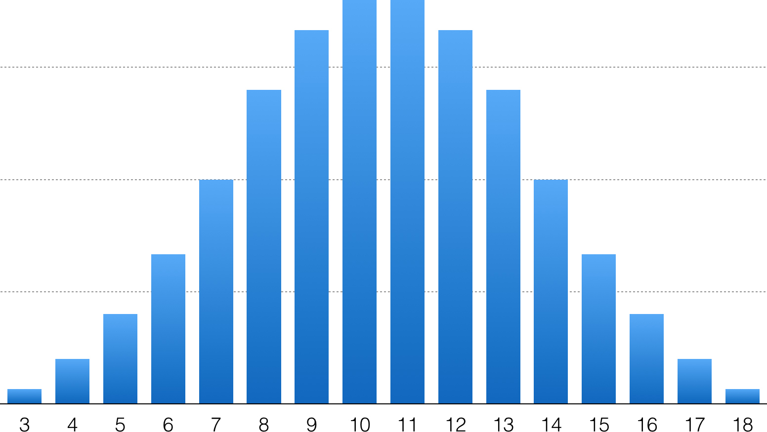
Figure 29.6 Probability distribution for 3d6.

This shows you that you cannot simply add dice rolls together and have the result be the same as a die of that many sides. For instance, as shown in Figure 29.7, 19d2 gives a result between 19 and 38, and also 1d20 + 18 gives a result between 19 and 38. However, 1d20 has a flat distribution. Any result happens just as often as any other. But 19d2 has a sharp curve with a high probability in the middle and low probabilities at the edges. The more independent die rolls you sum together, the steeper that curve will be. In 1d20 + 18, 19 happens 5 percent of the time because rolling a 1 on one die happens 5 percent of the time. But to get a 19 with 19d2 requires rolling a 1 19 times in a row, or 0.0002 percent of the time:

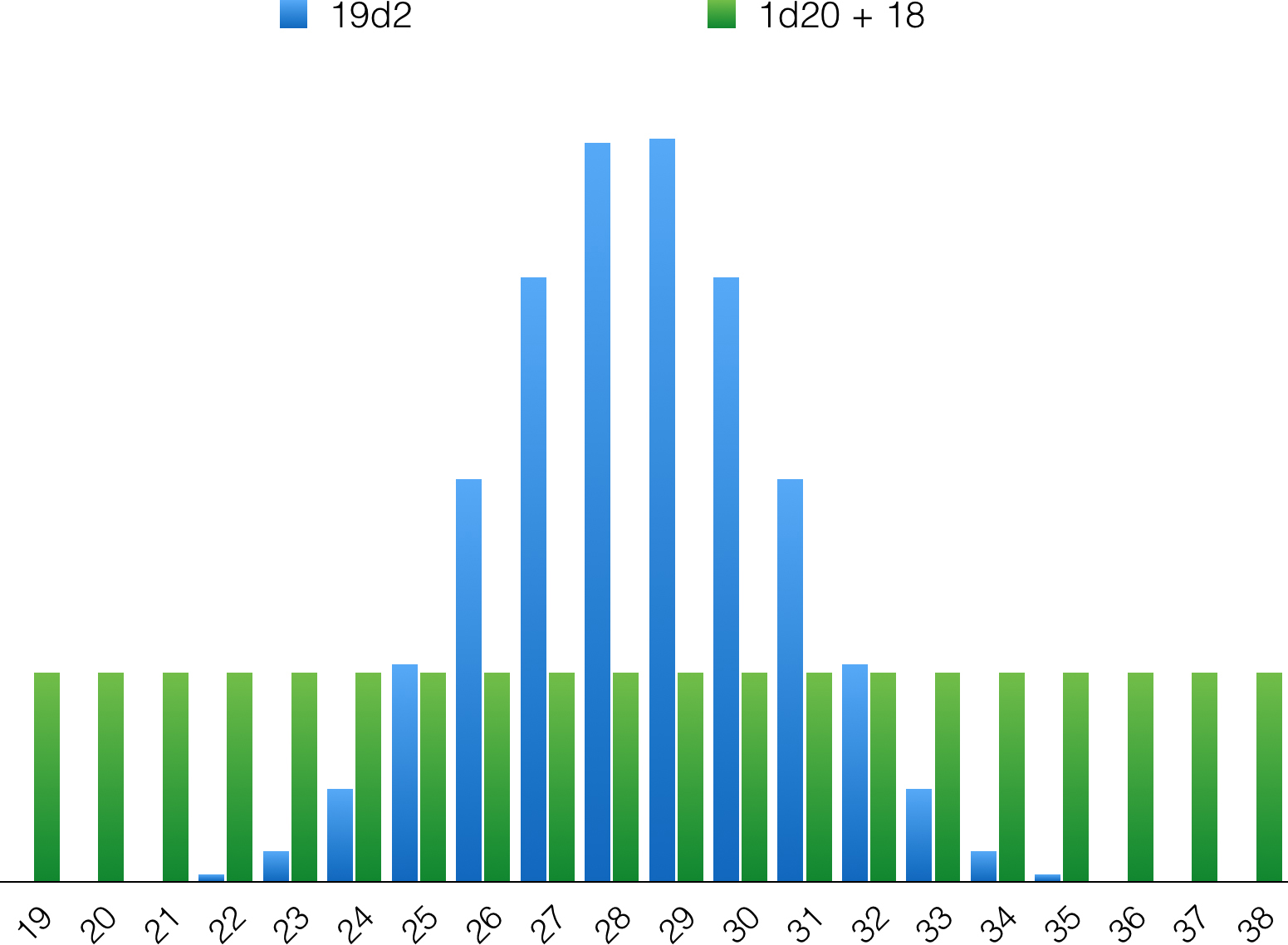
Figure 29.7 Although 19d2 and 1d20+18 have the same range, they have vastly different probability distributions.

Example: The H/T Game

Probability is often difficult to understand intuitively.

As an experiment, look at a simple game that I call the H/T game. In its basic form, the H/T game has two players. One of the players has a coin and flips it. If a player’s coin lands heads, he receives a point. If a player’s coin lands tails, the opponent receives a point. Players play for 1000 rounds. Yikes!

It would not be an interesting game to play, but its simplicity allows you to show how probability can fool us. The H/T game is probably the fairest game you can imagine. Each player has a 50 percent chance of winning each round. How often should the lead change from one player to the other?

Most people envision a series of coin flips like this:

THHTT HTHHT HTTHT THHHT

That looks pretty random. In 20 flips, it has 10 heads and 10 tails.

If this string represents the first 20 flips of the H/T game, tails would start winning on turn 1. Heads would start winning on turn 3. Tails would start winning again on turn 5. Heads would start winning on turn 9. On turn 13, tails starts winning again and keeps that lead until turn 19. This is represented in Table 29.1 and Figure 29.8.

Table 29.1 Lead Changes in a Run of the H/T Game

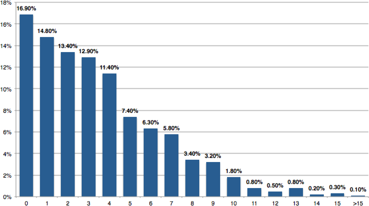
Figure 29.8 Simulation of lead changes in the H/T game with 1000 flips per game.

Twenty flips in this game have five lead changes. Since the probability of getting heads and tails is identical, the score difference should hover around 0 no matter how many times you flip, leading to a lot of lead changes. Twenty-five percent of the flips have a lead change. If you extrapolate to the 1000 flips you established earlier, then a reasonable guess for the number of lead changes should be something like 250. Certainly, it should be above 15 at a minimum, right?

Because my coin-flipping hand is slow, I decided to run a simulation of this game in Microsoft Excel. I had my computer play the H/T game 1000 times and count the number of lead changes (that is 1,000,000 flips!). Figure 29.8 shows the results.

One in 1000 games had more than 15 lead changes. Nothing ever even got remotely close to 250 lead changes. The most common number of lead changes was 0!

If you played the H/T game as the tails player and heads started winning and remained winning for all 1000 flips, you would likely get upset and assume that the coin was fixed. After all, with a fair coin, the number of flips should be even between heads and tails!

This is counterintuitive! This game has no feedback loops (Chapter 17). Having flipped a head previously does not increase or decrease the player’s odds of flipping another head. Yet in more than one in six games, a player takes the lead and never relinquishes it, even in an extremely long game.

This is just one example of how our instincts about probability can fool us. Be careful.

Being Careful

Probability can be tricky, as I’ll show with some additional examples. One of the ways not to be tricked is to be deliberate with your use of events and conditions, writing them down and charting them out rather than making assumptions. The first two problems that follow will show you how quick, “obvious” answers are anything but.

Problem #1: The Boy-Girl Problem

“I have two children. At least one of them is a boy. What is the probability that both are boys?”

Most people instinctively say that the probability is one-half. It’s irrelevant what gender the other boy is and that the question is only asking what the gender of other child is. Since you assume a 50/50 split between boys and girls, the odds that Child #2 is a boy is 1/2. Some will answer that since there are four possible permutations of gender in two children and only one of them is boy-boy, the answer must be 1/4.

This is a situation where it helps to slow down and be deliberate. There are four possible birth combinations: boy-boy, boy-girl, girl-boy, and girl-girl. However, we were told that one of these combinations is impossible. Girl-girl cannot be the result since we know that I have at least one boy (Figure 29.9).

Figure 29.9 The boy-girl problem.

This leaves us with three possibilities: girl-boy, boy-boy, and boy-girl. In those, only one meets the criteria that both are boys. So the answer is actually 1/3.

Problem #2: The Weirder Boy-Girl Problem

This version of the problem was posed by puzzle designer Gary Foshee. It looks roughly the same as the previous problem:

“I have two children. One is a boy born on a Tuesday. What is the probability that I have two boys?”

At first, it seems an absurd reduction of the first problem, so a knee-jerk answer would be “Also 1/3.” What would being born on a Tuesday have to do with gender probabilities?

The first thing to note is that our enumeration of all the possibilities is a lot more difficult than in the first problem. In that one, we had only four options. Now each of the four options has 49 sub-parts: 7 possibilities for Child 1’s birthday and 7 possibilities for Child 2’s birthday. This leads us to 7 * 7 * 4, or 196 possibilities (Figure 29.10).

Figure 29.10 Setting up the weirder boy-girl problem.

Each of the squares represents a possibility. For instance, if the first child is a girl, the second child is a boy and they are both born on a Friday, then the result is represented by the top-left table with the square that intersects F and F.

You must be careful about understanding what the question is asking. We know that one child is a boy born on a Tuesday. Given that, what is the probability that the other child is a boy? The question is asking for P(Other child is a boy | One child is a boy born on a Tuesday). When we found conditional probabilities earlier, we first highlighted the set from which we were counting. In this case, since we are given that one child is a boy born on a Tuesday, we first limit our counting to those squares. In the diagram, we can do this by highlighting them as in Figure 29.11.

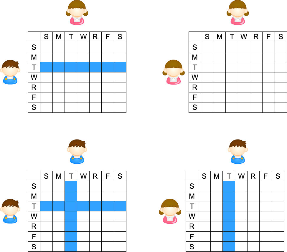
Figure 29.11 A step in the weirder boy-girl problem.

This is a total of 27 squares: 7 in the top-left table, 0 in the top-right table, 7 in the bottom-right table, and 13 in the bottom-left table. From these 27 squares, you want to know in which cases are both children boys? This part is easy. Only the squares in the bottom-left table. Since there are 13 squares there, the answer is 13/27.

You may be upset at this and ready to throw out the entire concept of probability, but wait. This problem does not say that having a boy on a Tuesday somehow changes the probability of having another boy. All it’s doing is giving you a fairly complicated statement of facts: I already have two children and here is a partial set of information about them. If I were to have a third child, the probability of that child being a boy or a girl would still be essentially 50/50.

It should also be noted that there are reasonable arguments that this is not the only solution, due to ambiguity of concepts.³

³ Khovanova, T. (2011). In “Martin Gardner’s Mistake.” Martin Gardner in the Twenty-First Century (p. 257). Washington, DC: Mathematical Association of America.

Problem #3: Isner–Mahut at Wimbledon

Wimbledon is a tournament of spectacle in the tennis world. However, it’s not often that a first-round match between a 23rd ranked player and an unranked qualifier player gets any immediate or subsequent attention. The 2010 Wimbledon first-round match between American John Isner and Frenchman Nicholas Mahut bucked that trend, setting records that will not easily be broken.

In major tennis tournaments, close matches are decided by tie-breaking games, except in the final set. In the final set, after playing a number of games and remaining tied, players must play until one player scores six games or more and wins two games in a row. Thus, a final set can be infinitely long in theory. Before 2010, the longest tie-breaking final set (in terms of games) went to a final score of 21–19 for a set of 40 games and a match length of 5 hours. Isner and Mahut’s match was played over three days because of lighting conditions, ending in a final score of Isner 70, Mahut 68 for a final set with 138 games. The match lasted a total of 11 hours and 5 minutes, nearly doubling the duration of the previous longest match in history (Figure 29.12).

ISNER & MAHUT, © SHUTTERSTOCK

Figure 29.12 Isner and Mahut pose after their record-breaking match.

If you wanted to model the probability of another match that rivaled the length of the Isner–Mahut match, you might start by assuming that the match lasted so long because the players were so evenly matched that each had a 50 percent chance of winning any game. Many commentators, such as those at the Daily Mail and the New York Times (among others) made such an observation.⁴,⁵

⁴ Harris, P. (2010, June 24). “Game, Sweat, Match! After 11 Hours, We Finally Have a Winner of the Longest Match.” Retrieved July 7, 2019 from www.dailymail.co.uk/news/article-1289130/WIMBLEDON-2010-John-Isner-Nicolas-Mahut-longest-tennis-match-ever.html.

⁵ Drape, J. (2010, June 23). “The Odds on How the Match Will Play Out.” Retrieved July 7, 2019, from www.nytimes.com/2010/06/24/sports/tennis/24betting.html.

Looking back at the H/T game, though, you know that flipping a series that perfectly alternates HTHTHTHT is very improbable. If it were as simple as Isner and Mahut being evenly matched, then by chance alone, one or the other would have lucked into a couple of “heads” coin flips in a row and ended the match. A series of 138 tosses that ended HTHTHT... or THTHTH... is so unlikely as to be impossible.

One element that a 50–50 assumption makes is that every game plays like every other. However, if you understand tennis, you know this is not true. The player who serves each game has an enormous advantage. This advantage is mitigated by alternating who serves on each game. To win two games in a row, the player has to win a game in which he serves, but he also has to win a game where he does not. Winning a game in which you do not serve is called “breaking serve” in tennis.

Making the assumption that the probability that Isner or Mahut wins any particular game is 50 percent assumes that the probability of either player breaking serve is also 50 percent. In a simulation of over 1000 matches that go to tiebreakers, if you assume a 50 percent break chance, no match exceeded 25 games, let alone approached 138 games. However, if the simulation is changed so that each player has a 25 percent chance of breaking serve, then the longest match jumps to 39 games. If each player has a 0 percent chance of breaking serve, no match would ever end because the serving player would always win and no player would ever break.

If you change the odds of breaking serve to 5 percent for each player, simulation results determine that one match in a 1000 reaches 138 games. With those odds, 31 percent of matches that go to tiebreakers still end before the 20th game. So even if Isner and Mahut were able to keep a huge 95 percent service win rate, they could play each other again and again and never see the marathon of Wimbledon 2010 happen again. I am sure they would be relieved to hear that.

The point of this example is that you need to be careful when you make assumptions about probability. Here, an assumption that a marathon game between two highly skilled opponents must mean that each has equal odds of winning each game shows a flaw in analysis that can ruin further assumptions about how the game will play out. A more careful analysis uncovers that it was not that Isner and Mahut were evenly matched, but that each was extremely highly skilled at keeping serve against the other on that day. Choosing the correct items to model leads to more valid projections and simulations.

Summary

• Probability is an essential mathematical tool for game designers. Those who shy away from math should be comforted in knowing that probability is just advanced counting.

• Joint probability can be found by multiplying the probability of two independent events.

• Conditional probability can be determined by dividing the joint probability by the probability of the given condition.

• Adding the probabilities of two random events can be challenging when they do not have a uniform distribution.

• Slowing down to enumerate the cases in a probability problem allows you to use simple methods to reach your conclusions.