31. Monte Carlo Simulation

All generalizations are false, including this one.

—MARK TWAIN

Games often rely on random number generation to determine the events of the game. The Monte Carlo simulation is a method in mathematics in which results are gleaned from trials generated by random numbers. By using the random number generation and manipulation within spreadsheet software, you can use the Monte Carlo simulation to answer fairly complex questions about how a game will behave.

It is often said that the Monte Carlo simulation is named after the roulette wheels of the Casino de Monte Carlo in Monaco. However, this is not entirely true. During World War II, scientists working on the atomic bomb needed to figure out a way to simulate neutron penetration for shielding purposes. Because it was a secret project, John von Neumann chose the loosely related name “Monte Carlo” for this method since it used random numbers; the name has persisted.

In this chapter, I’ll show some examples of how you can use the immense computational power of spreadsheets on modern computers, including how to simulate random elements in games in order to further answer questions about the effects of various game design decisions.

Answering Design Questions

The primary way game designers use Monte Carlo simulation is to quickly test how complex random events will act over time. Here is an example:

If a player hits the opponent with an attack four times in a row successfully, the fourth hit and each consecutive hit after is a super attack. The player can make 100 attacks per round. If the attacks hit or miss randomly at 50 percent and the designer wants to see 10 super attacks in a round, are there enough super attacks?

Creating a probability tree can solve this problem, but due to the size of the tree, it should be easier to solve this problem with a simple Monte Carlo simulation. To do this, you first need to understand what elements you need to track.

1. Make a list of the elements in the game.

• What is the number of attacks (it must be less than 100, since we established that there is a maximum of 100 per
round)?

• Does each attack hit?

• How many attacks in a row have hit?

• Is this attack a super attack?

2. Create a spreadsheet, and make a column for each item in the list, labeling them in row 1 as in Figure 31.1.

In the example here, I use two columns to answer the question about whether the attack hits. Column B rolls a random number, and column C evaluates that number, translating it into a hit or miss.

MICROSOFT CORPORATION.

Figure 31.1 Simulating super attacks.

3. Add the following data and formulas to the spreadsheet in row 2:

• Column A is a sequential number that indicates when I have reached 100 attacks. I called these “flips” in the header of the sheet just as a reminder that these are random events, like coin
flips.

• Column B is a randomly generated number. In B2, enter the formula =RAND().

• Column C answers whether that random number is good enough for a hit. It checks cell H1 (Figure 31.2) which is labeled “Hit Rate” and is set to 0.5 because the player hits 50 percent of attacks. In C2, enter the formula

=IF(RAND()<$H$1, "Hit", "Miss").

MICROSOFT CORPORATION.

Figure 31.2 How many?

• Column D is the trickiest one here. It checks column C to see if it is a hit. If it is, it adds 1 to the number above it to come up with its own entry. Otherwise, it sets itself back to 0. However, the first attack doesn’t have a previous attack to look at, so its formula cannot be the same as all the subsequent attacks. In D2, enter the formula =IF(C2="Hit",1,0). In D3, enter the formula =IF(C3="Hit",D2+1,0).

• Column E just prints out “Super” if the attack is a super attack. Otherwise, it leaves the cell empty. In E2, enter the formula

=IF(C2="Hit","Super","").

4. With all these in place, you can drag the contents down to repeat for 100 attacks.

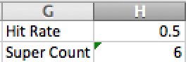
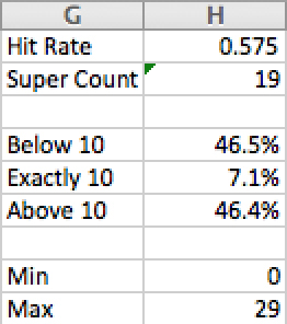
5. Column F is empty, just for readability. In column G, label one cell Hit Rate and another cell Super Count, as in Figure 31.2.

6. In H1, enter 0.5 for the hit rate.

This is a constant value for each attack.

7. In H2, enter the formula =COUNTIF(E2:E101,"Super"), which counts the number of times “Super” appears in column E.

This will give the answer to how many super attacks happened in that simulation.

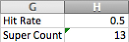
Figure 31.2 shows that the simulation ended with 6 super attacks, so it is way under schedule. However, this is really sensitive to fluctuation. By changing a cell somewhere else or by using the recalculate shortcut in Excel, you can run the simulation again and get drastically different results, as shown in Figure 31.3.

MICROSOFT CORPORATION.

Figure 31.3 Rerun the simulation, and you may get a very different result.

The problem is that 100 attacks are not enough to eliminate the variability of a 50 percent hit rate. One possible solution is to create a one-way data table that runs these 100 attacks over and over again.

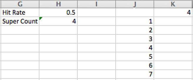
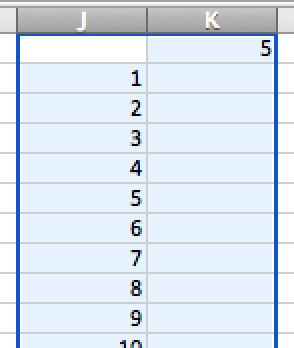
8. Create a reference in a new column (here I use K1; see Figure 31.4) to the Super Count value in H2, and list a trial number in column J up to 1000 trials. Remember from Chapter 30 that you need a dummy element that references what you want to reflect from each trial. Since you are looking for the number of super attacks in each trial, your dummy element in K1 simply points to the Super Count in H2.

MICROSOFT CORPORATION.

Figure 31.4 Setting up for a Monte Carlo simulation.

9. Highlight the entire table of trials (in this example, it is from J1:K1001; see Figure 31.5), and in Excel, choose to make a data table, selecting any empty cell as the column input.

MICROSOFT CORPORATION.

Figure 31.5 Highlighting for the data table.

This should give you a varying list of results for 1000 different 100-flip games. How many of these are above 10, and how many are below 10? By doing a COUNTIF on the results, you can determine that.

10. To determine the proportion of games that are below 10, enter the formula

=COUNTIF($K$2:$K$1001,"<10")/COUNT($K$2:$K$1001).

You can do this to calculate exactly 10 and above 10, similarly to Figure 31.6.

MICROSOFT CORPORATION.

Figure 31.6 Using COUNTIF.

Most of the time, there are fewer than 10 super attacks. Now that you have done all the leg work, you can change the Hit Rate cell (H1 in Figure 31.6) and try to find a hit rate where the number of super attacks above and below 10 are equal. A more robust solution is to make a two-way data table from the start where the hit rate fluctuates.

However, if you use a two-way data table, you must be sure to pick the hit rates to try carefully. As you will see, if you play with these numbers, the rate at which super attacks are above or below 10 is very sensitive. Fifty percent is far too low, but 60 percent is far too high. It turns out that when you nudge the hit rate from 0.5 to 0.575, the game sees the number of super attacks the designer desires. If you make a two-way data table and test only 10 percent, 20 percent, and 30 percent, and all the way up to 100 percent, you miss all the detail in the critical range between 50 percent and 60 percent.

The variability, however, remains high. By looking at the minimum value in the list of game results and the maximum value, you can see a range, as in Figure 31.7.

MICROSOFT CORPORATION.

Figure 31.7 Using MIN and MAX.

It may be that the design itself needs to be changed to address this variability if 0 or 29 are too low or high to be acceptable to the designer.

Hot Hand

In basketball, a player is said to have a “hot hand” if he has made some number of baskets in a row. The concept of the hot hand is that the player is more likely to make his next basket because he is hot. Similarly, a “cold hand” is when misses indicate that the player is likely to continue to miss.

You want to implement this feature in a basketball game you are making. Consider a player who has a base shot success rate of 50 percent. Every time the player makes three shots in a row, increase his percentage 10 percent (up to a maximum of 90 percent, because you never want shots to be automatic). Every time the player misses three in a row, his percentage drops by 10 percent (down to a minimum of 10 percent, because you never want shots to be impossible).

You can spend the time to code this into your game or you can run a simple Excel simulation. Draw a random number for each shot, determine if it is made or missed, and decide to adjust the probability for the next shot up or down (Figure 31.8).

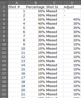
MICROSOFT CORPORATION.

Figure 31.8 Hot-hand simulation.

After 200 trials of 100 shots each, you can see a clustering of results (Figure 31.9).

MICROSOFT CORPORATION.

Figure 31.9 Hot-hand simulation end-value results.

After a while, the players converge to the hottest and coldest values. Once the player gets up to 90 percent, it’s unlikely he’ll ever miss three in a row to get colder. Conversely, once a player gets down to 10 percent, it’s unlikely he’ll ever hit three in a row to boost his percentage. With a couple of minutes of work, you can see that you need to either change your numbers or drastically rethink the feature.

By the way, researchers have shown that the “hot hand” phenomenon does not exist in basketball and that it is just an artifact of people misunderstanding randomness.¹

¹ Gilovich, T., Vallone, R., & Tversky, A. (1985). “The Hot Hand in Basketball: On the Misperception of Random Sequences.” Cognitive Psychology, 17(3), 295–314.

Monty Hall

Marilyn vos Savant writes a column for Parade magazine in which she solves puzzles and other questions. A September 1990 edition of her column caused an uproar when she was posed what is called the “Monty Hall Problem”:

Suppose you’re on a game show, and you’re given the choice of three doors: Behind one door is a car; behind the others, goats. You pick a door—say, No. 1—and the host, who knows what is behind the other doors, opens another door—say, No. 3, which has a goat (Figure 31.10). He then says to you, “Do you want to pick door No. 2?” Is it to your advantage to take the switch?

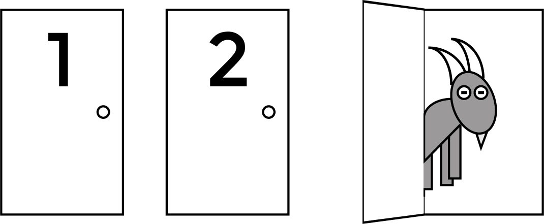
Figure 31.10 Monty Hall problem.

Marilyn answered that the correct strategy is to switch, because a switch provides a win 66 percent of the time. Thousands of angry letters flooded into the Parade offices, including many letters from readers with PhDs from prestigious mathematics departments who insisted that switching or not switching should each have a 50 percent chance of winning.² This makes initial sense. The prize is between one of two remaining doors, so the odds of winning when switching must be 50 percent. Who is right?

² Tierney, J. (1991, July 20). “Behind Monty Hall’s Doors: Puzzle, Debate and Answer?” Retrieved July 8, 2019, from www.nytimes.com/1991/07/21/us/behind-monty-hall-s-doors-puzzle-debate-and-answer.html.

You don’t need to be a mathematics PhD to solve this. You need only a spreadsheet and some ability to perform a simulation (Figure 31.11).

MICROSOFT CORPORATION.

Figure 31.11 Setting up Monty Hall.

In column B, a simple formula, =RANDBETWEEN(1,3), chooses a random door for the prize. The same formula works for the player choosing a random door.

The only difficult part here is understanding which door Monty will reveal (Figure 31.12).

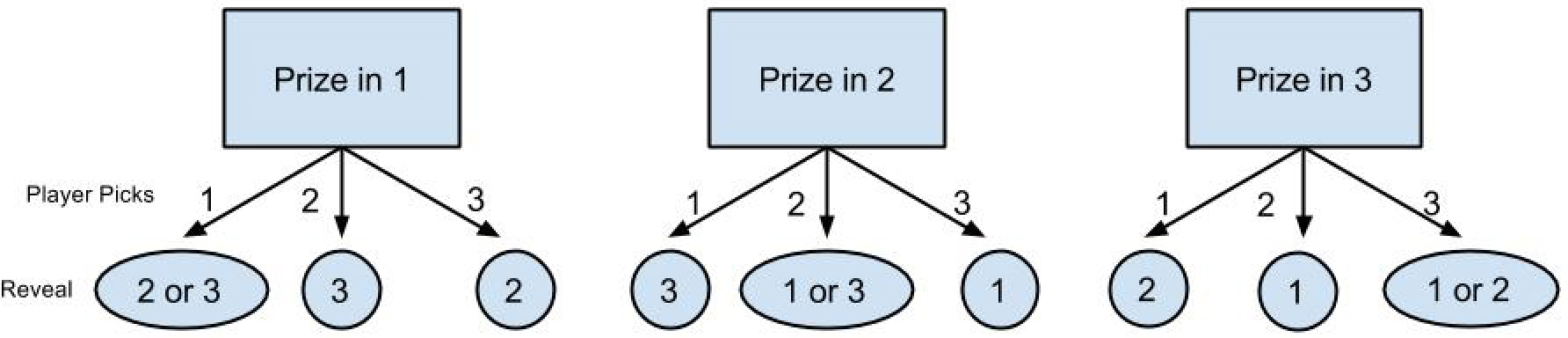
Figure 31.12 Diagramming the logic helps visualize the problem.

You do not actually need to understand which door Monty will open, though! Does it matter what door the player sees? Column E uses an IF statement to output “Win” if columns B and C are the same. All that’s left to do is count the frequency of Wins: It should be around 0.66.

Marilyn’s naysayers would say that it does matter what door you are shown, so I should probably go through with the exercise.

Which door will be opened? If you know two of the door numbers (1, 2, or 3) and know that they are different, then the third door must be neither of those since there are only three doors. You don’t need a complicated formula for this. The three door numbers sum up to 6 (1+2+3) no matter in what order they are placed. If you know two of the door numbers, then you can calculate the number of the remaining door as 6 – DoorOne – DoorTwo. If the randomly chosen door and the randomly assigned prize door are the same, then it doesn’t matter which of the remaining doors the host reveals.

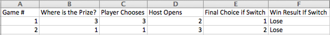
To check if switching results in a win, see if 6 – ChosenDoor – RevealedDoor equals the door number where the prize is (Figure 31.13).

MICROSOFT CORPORATION.

Figure 31.13 Runs of Monty Hall.

Now drag the cells down to create more runs of the game. (In this example, I chose to use 5000 trials.) Next, create a cell that does a COUNTIF on the Win Result If Switch column and looks for Win. Divide that by the number of trials, and you have the odds that switching will result in winning the prize. In this example, the spreadsheet calculated a 66.7 percent chance of winning if switching, just as Marilyn said!

Example: Dungeons & Dragons Advantage/Disadvantage

Players of Dungeons & Dragons generally determine random events by rolling dice. If the number rolled meets or exceeds a target number, then they succeed. Otherwise, they fail. In Dungeons & Dragons 5^TH Edition, players have to deal with a new mechanic, named “advantage and disadvantage.”³ With this mechanic, if the player is in a situation in which the character has a higher-than-normal likelihood of succeeding, she rolls two dice and takes the higher number. This is “advantage.” If the player is in a situation in which the character should have a lower-than-normal chance of succeeding, she rolls two dice and takes the lower number.

³ Wizard’s RPG Team. (2014). Dungeons and Dragons Player’s Handbook (5th ed.). Renton, Washington: Wizards of the Coast.

Game designers can use simulation to determine the effect of this mechanic on successes and failures. Before Dungeons & Dragons used the advantage/disadvantage system, a way to increase or decrease difficulty was to have a bonus or penalty based on a roll. For instance, if something was difficult, the player may have had to subtract 3 from her roll. Does “advantage” give too much advantage? How much does it give when compared to the old system? This is something that can be easily modeled in a spreadsheet.

1. Open your spreadsheet of choice, and create headings to organize the data, as in Figure 31.14.

MICROSOFT CORPORATION.

Figure 31.14 One set of rolls using all three systems.

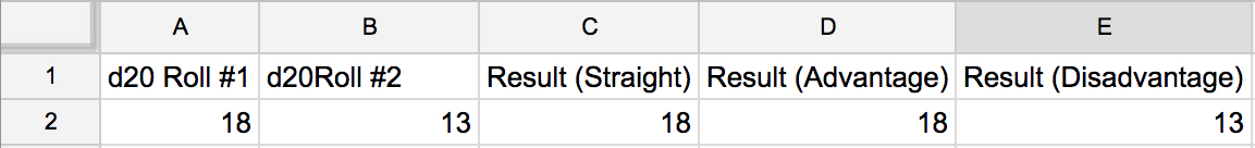
I have created headings to track die rolls (two are needed because the advantage/disadvantage mechanic uses two rolls), and the results. A d20 roll is a 20-sided dice. This can be done by taking a random number between 0 and 1 and multiplying by 20 and then rounding up to the nearest integer. This gives a random number between 1 and 20. However, most spreadsheets have a RANDBETWEEN function, so it is easier to use that.

The “straight” result would be to just take the first die roll.

2. In column C, enter the formula =$A2.

The “advantage” result would be to take the higher result.

3. In column D, enter the formula =MAX($A2,$B2).

Likewise, the “disadvantage” result takes the lower result.

4. In column E, enter the formula =MIN($A2,$B2).

5. Highlight the cells with the formulas you just entered, and drag down to copy them to 1000 repetitions.

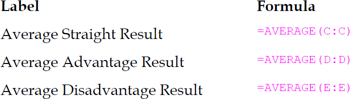
Now, by using the =AVERAGE function, you can calculate the average result for straight, advantage, and disadvantage.

6. Use columns G and H to label and calculate the straight, advantage, and disadvantage averages (Figure 31.15):

MICROSOFT CORPORATION.

Figure 31.15 Summary statistics. It makes sense for the average straight result to be 10.5.

The average result for a straight roll is easy to visualize. Since every side on a 20-sided die should come up with even frequency, the average should be (1+2+3+...+20)/20, or 10.5. If your average is much different than that (below 10 or above 11), keep rolling dice or check your math.

In the trial, the straight result’s average was 10.51, which was expected. The average “advantage” roll resulted in a 13.86 or a 3.34 difference to the straight result. The average “disadvantage” roll resulted in a 3.30 difference to the straight roll. Thus, you can say that the “advantage” system is somewhat equivalent to the old system of adding 3.3 to a d20 roll and the “disadvantage” system is somewhat equivalent to subtracting 3.3 from a roll.

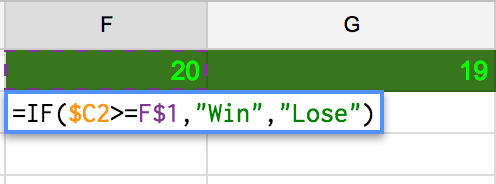
To go further, you can check each row against success of a target value to generate a win or loss for each value. Then, by counting wins versus losses, you can generate a table of probabilities for each technique for each target value (Figure 31.16).

MICROSOFT CORPORATION.

Figure 31.16 Checking against a target value in F$1.

Most spreadsheets recalculate all cells every time a cell changes. Thus, large spreadsheets with many calculations (as in this exercise) can result in a slowly running spreadsheet, so be careful to change a cell only when you can wait for the recalculations. Excel allows users to change a sheet’s preferences so that it recalculates only on a particular key press, which lets a user decide when the sheet should crank out the calculations. Google Sheets, at the time of this writing, does not have this setting.

Check the results in Figure 31.17 of simulating every difficulty under the three conditions. You know that each step on the Straight column should increase the probability by 5 percent, since each side has an even 5 percent chance of showing up. Since this is a simulation, there will be some variability. But more or less, it meets expectations.

MICROSOFT CORPORATION.

Figure 31.17 Probabilities of winning against stated difficulties in all three systems.

This is a better way of evaluating the advantage/disadvantage system because it answers more questions than the previous evaluation. Now you can see exactly how different the probabilities are under each condition for each difficulty level.

For instance, a difficulty of 15 has a 50 percent chance of a successful attempt under an advantage roll, but has a less than 10 percent chance when rolling disadvantage. The previous + or –3 is a good rule-of-thumb analysis for the difficulties near the middle of the spectrum, but as you can see, when you chart the probabilities (Figure 31.18), all types converge at the top and bottom and diverge toward the middle.

MICROSOFT CORPORATION.

Figure 31.18 The same probabilities graphed.

All of this can be done using spreadsheets on just a simple mechanic.

Once Around the Board

The ABC television network aired a Monopoly game show for a short time in 1990. It followed the traditions of normal game shows while being somewhat Monopoly-themed. One of the contestants would win the main part of the episode, and then get a chance to win additional prize money in the bonus round called “Once Around the Board.”

In the bonus round, the goal was to start the player’s pawn at Go and make an entire lap around the Monopoly board. But before the round began, the contestant had to choose four spaces on the board to transform into “Go to Jail” spaces. One space had to be placed in the maroon/orange properties, one on the red/yellow properties and two on the green/blue properties. So in addition to the traditional “Go to Jail” space, there were five spaces on the board where the player would automatically lose.

The player had five rolls to complete the circuit but would get a bonus roll if he rolled doubles. If the player quit or ran out of turns without hitting a “Go To Jail” space, then he would win $100 per space cleared. If he passed Go, he would win $25,000. If he landed on Go, he would win $50,000.

Assuming the player never chooses to quit early, and assuming that the properties in each block where the player must choose to place an extra “Go to Jail” occur with the same probability, what are the probabilities of winning? Say you are working for the producers of this show, and they can only afford to give away an average of $12,000 per episode. Is this a good design for that limitation?

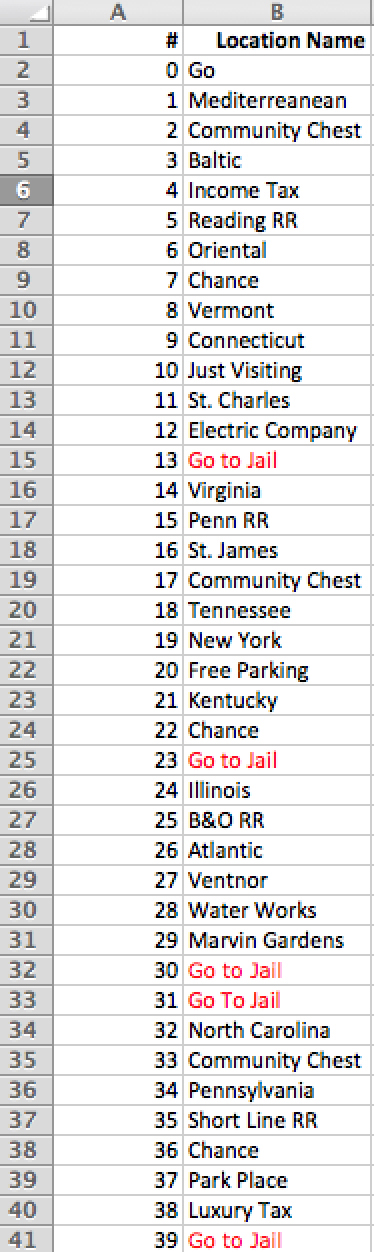
First, I created a list of all the locations in the game in the order they appear on the board. Since I assume that each location that can receive a “Go to Jail” space happens with the same probability, I can choose any four that meet the requirements and call them “Go to Jail,” as in Figure 31.19. The names are not a requirement for this to work, but it can help with readability.

MICROSOFT CORPORATION.

Figure 31.19 Mapping locations to numbers.

Next, I need to keep track of where the player lands. Remember that in the dice roll, the player rolls two 6-sided dice. This is a different distribution than one 12-sided dice (remember from Chapter 29), so I didn’t put =RANDBETWEEN(1,12). Instead, I used two separate =RANDBETWEEN(1,6) columns. Since I need to check for doubles (when the numbers rolled on the dice match), having two separate columns for dice is helpful, as opposed to one column with =RANDBETWEEN(1,6)+RANDBETWEEN(1,6).

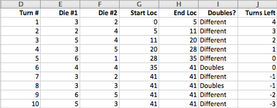
It is highly unlikely that the player will roll enough doubles of a low number that the game will not end by the eleventh turn, so I simulate 10 rolls. I also need to track the player’s start position on each turn so that I know where on the board he lands. I also need to know how many rolls the player has left (Figure 31.20).

MICROSOFT CORPORATION.

Figure 31.20 Simulating turns.

I determine the end location by adding the two dice the player rolled to the start location. I also set up a check for whether the location ends up being greater than 40. For anything after passing Go (>40), I have the spreadsheet return the value 41. Remember that for this game, we do not care about positions beyond the player reaching Go.

Doubles are calculated with an IF statement that says that if column E is equal to column F, then the player rolled doubles. “Turns Left” represents how many turns the player has remaining after that roll. On the first row, I check whether the player rolled doubles that turn. If so, it stays at 5; if not, it goes to 4. On each subsequent row, I check for doubles and either repeat or decrement the row above.

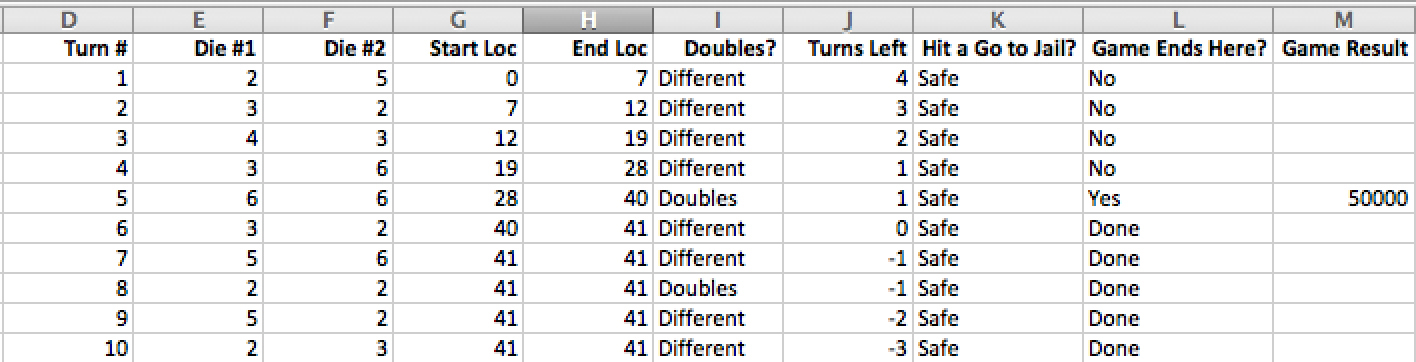
In the “Hit a Go to Jail?” column, I want to know if the player has hit a “Go to Jail” spot on this roll, so I just check whether the end location number matches one of the locations that say “Go to Jail” listed in column B.

Now it gets a little tricky. I want to know if the game ends on a particular throw (Figure 31.21). That way, I can calculate the result for the game. If I do not do this, then I have no idea which throw to use to calculate the result of that game. For instance, if a player landed on Go to Jail on one throw and then on Go on the next (since I always calculate ten throws win or lose), how would the game know whether the result was $0 or $50,000?

MICROSOFT CORPORATION.

Figure 31.21 Determining game end.

It helps to write out these conditions as a flowchart (Figure 31.22). There are three possible outcomes: The game ends on this turn, the game has already ended, or none of the conditions have been met and the game is still going. If I have only two conditions (the game ends this turn; the game does not end this turn), then the sheet thinks that the game can restart.

Figure 31.22 Flowchart for determining whether or not the game is over on this turn.

I make a flowchart because the spreadsheets allow for only one crowded line of nested IF statements. This allows me to make sure I have not missed any cases. It is easier to read than the following formula (Figure 31.23):

=IF(OR(L2="Yes",L2="Done"),"Done",IF(K3="Jail","Yes",IF(J3=0,"Yes",
IF(H3>39,"Yes","No"))))

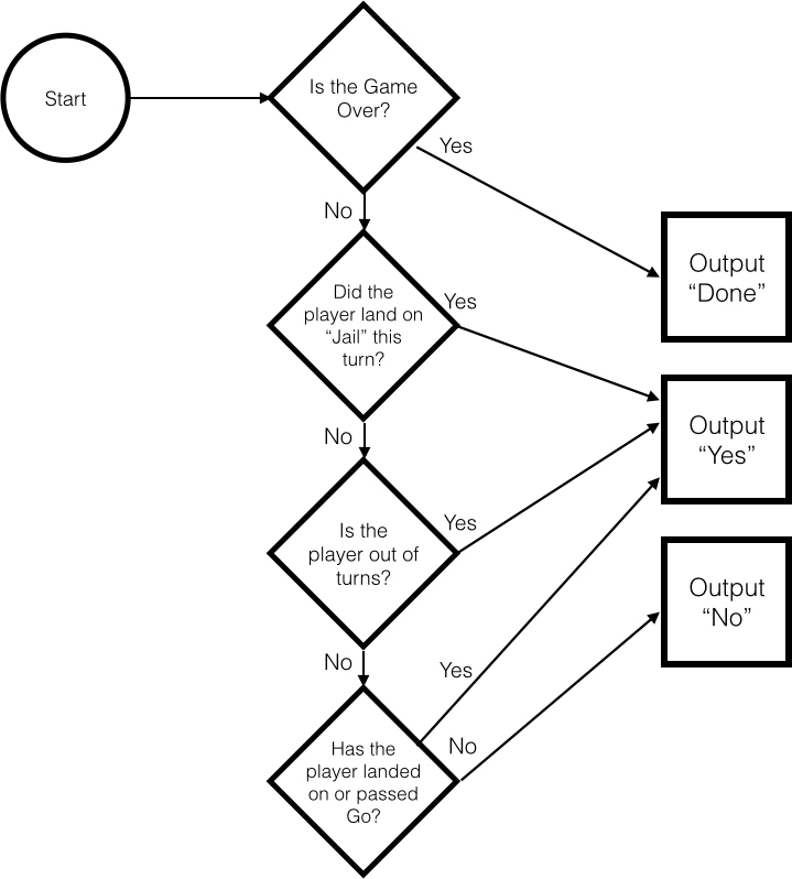
Figure 31.23 A complicated formula can be difficult to trace.

The final column is easier and is represented by the flowchart in Figure 31.24. If the result in the previous column is Yes, then calculate the winnings. Only one row can be Yes. Every other row must be Done or No, so this should give only one result for the whole table. When the game is not over, I have the cell output “”— nothing is outputting. That way, when I sum all the cells in this column, I end up with the game result. This also works if you have it output 0, but the null (two quotation marks indicating no character) looks cleaner.

Figure 31.24 Flowchart for determining the final value.

This process results in only one number popping up in the column for each game. From this, I can generate a data table of game results and then calculate the summary statistics or create a graph (Figure 31.25).

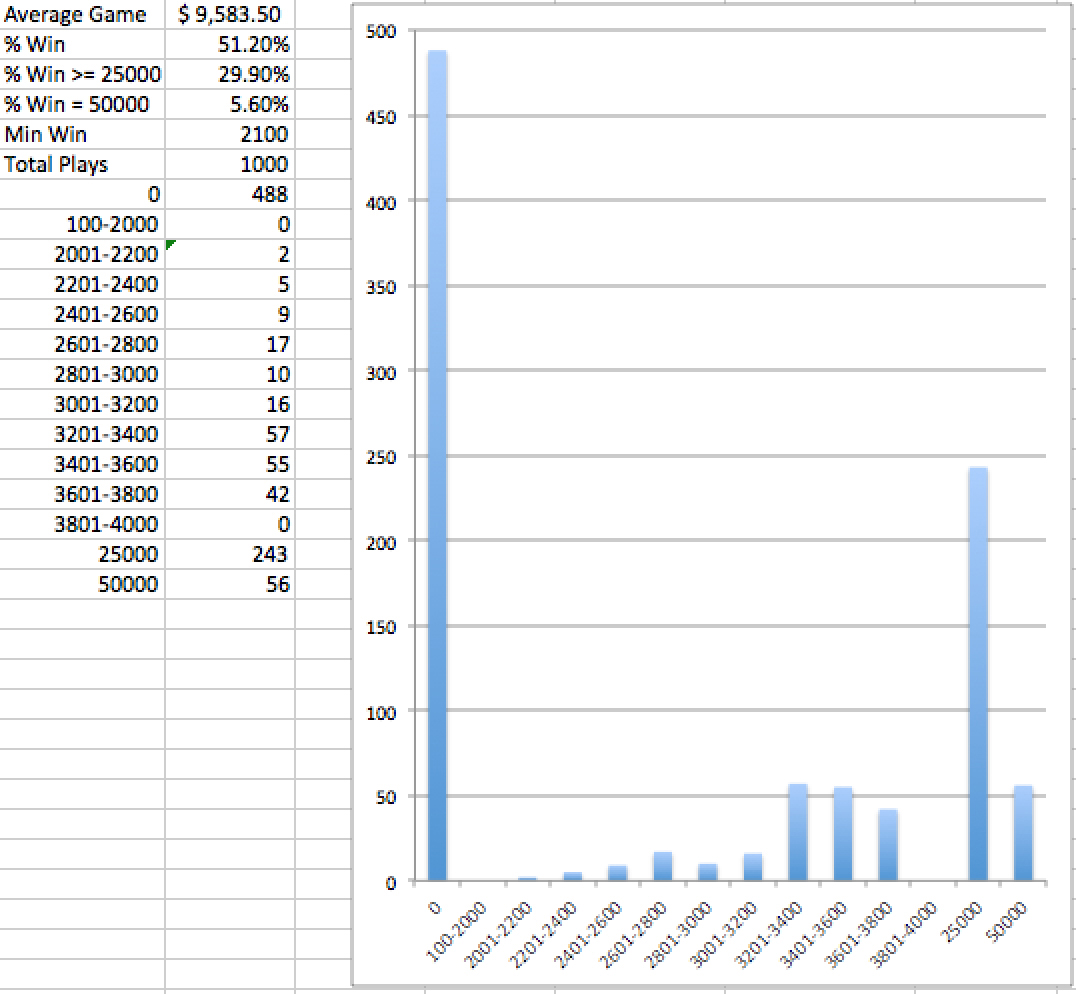
MICROSOFT CORPORATION.

Figure 31.25 Simulated “Once Around the Board” games.

The original question was to find out whether the game would cost the producers more than $12,000 per episode. Over 1000 games, this is not likely. Considering that there were only 13 episodes of the actual Monopoly game show, it was possible that all the wins would cluster in the first 13 shows. You can use this spreadsheet to determine the number of times that would happen. This analysis is great to show the producers because it answers many other questions. For instance, the producers probably do not want a final round to never end in a win, because that would make for bad television. However, they also do not want a final round that gives away too much money. This analysis shows the producers exactly how often the players win and how much they win.

Martingale Betting

Gamblers like to believe they can develop systems to beat the odds. One such system that has been around since at least the 18th century is known as the martingale betting system. In it, a gambler bets a set amount. If she loses it, she bets double on the next game. If she wins that game, then she is back to the starting amount and she resets the bet back to the original amount. Otherwise, she keeps doubling the bet. Theoretically, the gambler is bound to win eventually, and thus she should always be able to return to her original pot size.

Does this actually work? Let’s bias in favor of the gambler and provide a game with a 50 percent win rate. This is obviously better odds than you receive in a casino. Further, let’s give the gambler humble aims. The gambler enters the casino with $100 in her pocket. She leaves either when she has enough money to pay for a satisfying sandwich on the house (+$10) or is bankrupt.

This is a simple simulation. The columns of the sheet should start with a game number, a balance, a bet for that game, a result for that game, and a balance for after the game is complete. Additionally, a column should indicate if either of the terminating conditions has been reached (Bankrupt or Sandwich) (Figure 31.26).

MICROSOFT CORPORATION.

Figure 31.26 Martingale simulation setup.

Each row checks the balance of the previous row. The first row is different since there are no previous games to check. The bet is set to 0 if one of the terminating conditions has been met, ending the game. If the player gets to $0 or $100, then the game sets the terminating condition. Running this once is interesting. But running this for a year’s worth of “days” of games is better. Of those 365 days, how many days does the gambler get a sandwich and how many days does she lose all $100 (Figure 31.27)?

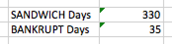
MICROSOFT CORPORATION.

Figure 31.27 The results are 35 bankruptcies if you walk in with $100.

This looks pretty good! The gambler has roughly a 90 percent chance of getting a “free” $10 sandwich and a 10 percent chance of losing $100. The expected value here is roughly 0. But what happens if I change the amount the gambler walks in with to $500 (Figure 31.28)?

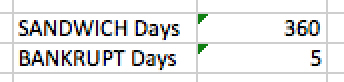
MICROSOFT CORPORATION.

Figure 31.28 The results are five bankruptcies if you walk in with $500.

Since the gambler’s pockets are deeper, she goes bankrupt less often. But now for five days in the year, she is paying $500 for her otherwise “free” sandwich! The expected value of playing the game goes from $0 to negative $3.83 per day. This is, of course, examining the situation from a rational, risk-neutral perspective. What happens if the gambler racks up two bankrupt days on her first two tries? She has now paid $1000 for no lunch at all.

Let us increase the amount the gambler starts with one more time. Now she comes in with $5000 (Figure 31.29).

MICROSOFT CORPORATION.

Figure 31.29 The results are two expensive bankruptcies if the player walks in with $5000.

Most days, she has no problem getting a sandwich. Those very deep pockets mean that she rarely has to double to the point at which she may lose her purse. However, on two days that year, she did lose out and paid $5000 for no sandwich. The average losses that year were negative $17.45 per day!

Besides having a limited pool of money from which to draw, another reason that martingale betting systems are not feasible is that casinos often limit the amount you can bet. Thus, if our $500 gambler needs to bet $64 to get back to break-even, she might be limited to betting $50, thus capping her ability to climb back out of the hole.

The martingale betting system follows the form of what is sometimes called a “Taleb distribution,” named after the author of The Black Swan, Nassim Nicholas Taleb.⁴ In a Taleb distribution, most of the results offer a nice, steady return. But every once in a while, the bet can go extremely poorly and wipe the bettor out. Choosing sample returns to evaluate something in a Taleb distribution is misleading. If you took 10 sample days from the $5000 martingale example, you would likely end up with ten “SANDWICH” days, leading you to believe that the betting system is foolproof. This is sometimes cited as the framework that is partially responsible for the great financial crisis in 2008: Firms took bets on items with extreme tail risk but evaluated them in terms of the risk of the non-tail results.⁵ This is like evaluating the martingale betting system described earlier by looking at the proportion of the SANDWICH days and not looking at the probability and impact of the BANKRUPT days.

⁴ Taleb, N. N. (2010). The Black Swan: The Impact of the Highly Improbable (Vol. 2). New York, NY: Random House.

⁵ Taleb, N. N. (2010). “Why did the Crisis of 2008 Happen?” DRAFT, 3RD Version. Retrieved July 8, 2019 from www.fooledbyrandomness.com/crisis.pdf.

In games, this is important because it is the edge cases that break a system. If a multiplayer game’s economy works for 99 of 100 players, what impact does that 100th player have? Discounting him because of his low probability is not wise, just as discounting the low probability of BANKRUPT days on the $5000 martingale example is not wise.

Summary

• There is wide applicability of Monte Carlo simulations for answering design questions.

• Be careful about how your chosen number of trials affects the variability of your results. If your summary statistics jump around a good deal from one simulation of trials to the next, you may not be using enough trials in your simulation.

• Drawing out flowcharts for complicated steps can help ensure that you are accurately defining all the steps you need for difficult calculations.

• Often, elements of your simulation vary by different amounts with respect to your inputs. By choosing a wide range of inputs to examine, you can be sure not to miss interesting behaviors that happen outside your simulated results.

• You must carefully examine distributions with large events in the tail. Sampling too few events without understanding the tail risk can lead to misinterpreted results.