
Chapter 4: Describing Two Variables at a Time
Describing Covariation: Two Categorical Variables
A Digression: Recoding a Variable and Changing Value Order
Describing Covariation: One Continuous, One Categorical Variable
Describing Covariation: Two Continuous Variables
Scatter Plots for Very Large Data Tables
More Informative Scatter Plots
Some of the most interesting questions in statistical inquiries involve covariation: how does one variable change when another variable changes? After working through the examples in this chapter, you will know some basic approaches to bivariate analysis, that is, the analysis of two variables at a time.
Chapter 3 covered techniques for summarizing the variation of a single variable: Univariate distributions. In many statistical investigations, we are interested in how two variables vary together and, in particular, how one variable varies in response to the other. For example, nutritionists might ask how consumption of carbohydrates affects weight loss or marketers might ask whether a demographic group responds positively to an advertising strategy. In these cases, it’s not sufficient to look at one univariate distribution or even to look at the variation in each of two key variables separately. We need methods to describe the covariation of bivariate data, which is to say we need methods to summarize the ways in which two variables vary together.
The organization of this chapter is simple. We have been classifying data as categorical or continuous. If we focus on two variables in a study and conceive of one variable as a response to the other factor, there are four possible combinations to consider, shown in Table 4.1. The next three sections discuss three of the four possibilities: We might have two categorical variables, two continuous variables, a continuous response with a categorical factor, or a categorical response to a continuous factor.
Table 4.1: Chapter Organization—Bivariate Factor-Response Combinations
|
Continuous Factor |
Categorical Factor |
|
|
Continuous Response |
Third section to follow |
Second section to follow |
|
Categorical Response |
See Chapter 19 |
Next Section |
In this chapter, we will introduce several common methods for three ways to pair bivariate data. The first examples relate to a serious issue in civil (non-military) air travel: the periodic collisions between wildlife and commercial airplanes. According to the U.S. Federal Aviation Administration (FAA) so-called wildlife-aircraft strikes have cost hundreds of lives in the past century and account for significant financial losses as well in damage to aircraft. These collisions present environmental, public safety, and business issues for many interested parties. The FAA maintains a database to monitor the incidence of wildlife-aircraft strikes. From 2010 through April 2019, the database contains nearly 117,000 reports of strikes in North America. The state reporting the largest number of events was California.
For this chapter, we will use a subset of the database, looking only at bird strikes associated with three California airports: Los Angeles International, Sacramento (the state capital), and San Francisco International. All of the available data is in the data table called FAA Bird Strikes CA. This data table contains 36 columns providing attributes for each of 3,411 bird strikes at or near the three airports.
1. Open the FAA Bird Strikes CA data table now and scroll through the columns. Our analysis will use several columns, each of which we will explain as we work through the examples.
The REMARKS column in this data table has an icon that we have not previously seen: ![]() This column contains Unstructured Text, which is free-form character data. Specifically, remarks are the written description of the wildlife strike as provided by the person who filed the original report.
This column contains Unstructured Text, which is free-form character data. Specifically, remarks are the written description of the wildlife strike as provided by the person who filed the original report.
Although it is well beyond the scope of this book, interested readers should check out the Text Explorer platform in the Analyze menu or visit www.jmp.com for demonstrations and examples of text analysis.
This data table also has a large amount of missing data. Although the FAA attempts to record a full set of variables for each strike, sometimes the data is not known to the individual reporting the incident. In a JMP data table, missing categorical data appears as a blank cell, and missing continuous data is a dot.
In a bivariate analysis, we think in terms of a pair of observations for each bird strike. JMP will only analyze those incidents that have a complete pair of observations for whichever two columns that we select.
Describing Covariation: Two Categorical Variables
At what point in a flight do bird strikes most often occur? Was it the same at all three airports? In our data table, we have two variables that identify the airport (the Airport code and City) and another ordinal variable identifying the Phase of the Flight at which the strike happened. We can use JMP to investigate the covariation of these categorical variables using a few different approaches.
1. Select Analyze ► Distribution. You should be quite familiar with this dialog box by now. Select the AIRPORT and PHASE_OF_FLT (phase of flight) columns, cast them into the Y role, and click OK.
JMP produces two univariate graphs with accompanying frequency tables for each of the two columns. In the default state, they reveal no information about patterns of covariation, but there are a few important things to notice. Look at the phase of flight data and see that several of the levels of this column are repeated, but with different capitalization. Our analysis will be simplified if we can treat APPROACH and Approach as the same thing.
A Digression: Recoding a Variable and Changing Value Order
When data are recorded by many individuals over a long time period, sometimes variations in spelling, punctuation, or capitalization creep into a set of data. Prior to analysis, we typically want to clean up and standardize such variation when we find it.
1. Make the data table the active tab of your project and select the column PHASE_OF_FLT.
2. Select Cols ► Recode. The Recode dialog box (Figure 4.1) lets us replace current values with new ones.
Figure 4.1: Recode Dialog Box
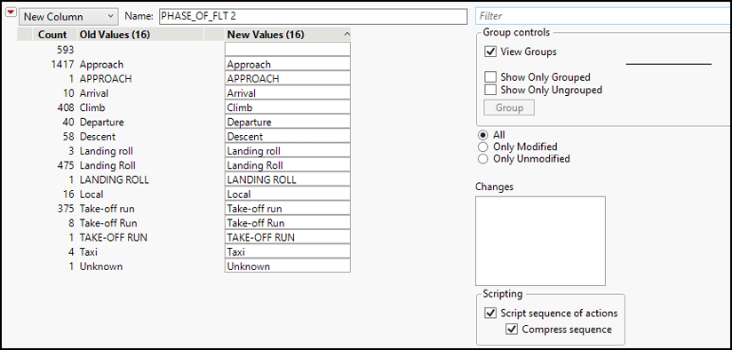
We have the option to preserve the original data and create a new column, and then individually type in text to replace values that we want to standardize. In this case, we see that 1,417 incidents happened on Approach and 1 happened on APPROACH.
3. In the New Values (16) column, replace APPROACH with Approach. Notice the changes in the dialog box that indicate that two old values that were previously treated as different are now grouped together.
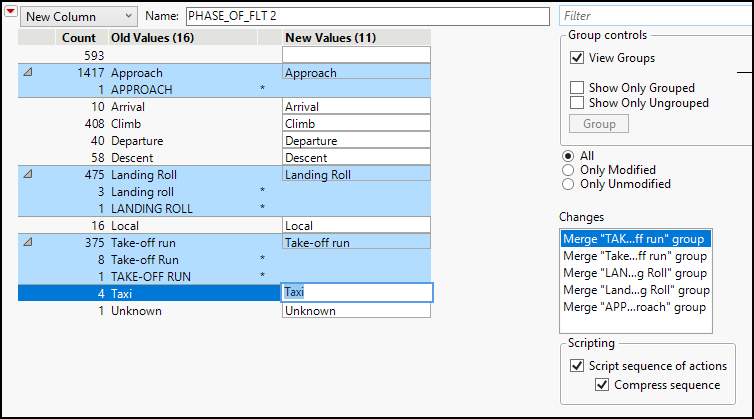
4. Continue by recoding all the Landing Roll and Take-off run levels. When finished, your dialog box should look like Figure 4.2. Then click Recode.
Figure 4.2: Recoded Values
Also notice that the flight phase values are in alphabetical order. It might be more useful to change the order to correspond to the chronology of a flight, and fortunately this is easy to do. The basic chronology of the phases in this data table is as follows:
● Departure
● Taxi (the FAA distinguishes between Taxi-out and Taxi-in, but here we just have “Taxi”, which occurs 4 times)
● Take-off run
● Climb
● Descent
● Approach
● Landing Roll
● Arrival
● Local (rare; apparently refers to strikes noted at an airport)
● Unknown
5. In the Columns pane of the data window, right-click on the column PHASE_OF_FLT 2 and select Column info…
6. Click Column Properties and select Value Order.
7. As shown in Figure 4.3, highlight Departure in the Custom Order list of values, and use the black arrows to move it to precede Approach. Note the blank line above Approach, representing missing values. We can leave that as the first item in the list.
Figure 4.3: Defining a Custom Value Order
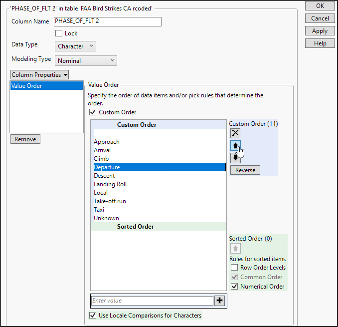
8. Continue using the up and down arrows to place the value labels in the desired order. When you finish, click OK.
Back to the bivariate analysis
1. Again, select Analyze ► Distribution and cast AIRPORT and PHASE_OF_FLT 2 columns into the Y role, and click OK.
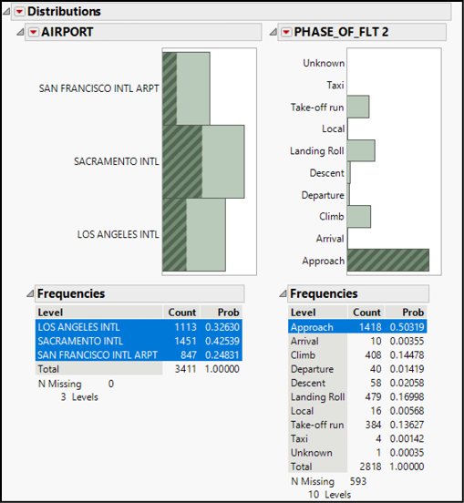
Wildlife strikes are rare during the taxi phase (in either direction between the terminal and runway) and Arrival phase. We also should note that, although the FAA database does contain strike reports while flights are en route, these three airports did not report any such strikes. Consequently, the en route phase of flight does not even appear in the right-hand panel of this graph.
In contrast, more than 50% of the strikes occurred during the approach phase of the flight. Clicking the Approach bar highlights the bar in the right-hand graph and also highlights all approach-related observations in the left-hand graph. If the relevant dynamics are similar at the three airports, then we would expect approximately half of each of the three bars in the left chart to be darkened. However, this is not the case. We will explore this curious pattern shortly.
2. Click the bar representing Approach (to the airport just prior to landing), we see something interesting, as shown in Figure 4.4.
Before going further, look at the frequency tables under each graph. Each table tallies the number of observations in each column category as well as the number of missing observations, and the number of distinct values (levels) within the column. The data table identifies the airport city for every bird strike, but only has data about the flight phase for 2,818 incidents. The other 593 are missing—they are unknown to history.
Figure 4.4: Two Linked Univariate Distributions
The issue of missing data is quite common in observational and survey data, though introductory courses often bypass it as a topic. In a bivariate analysis, we will need two values for each observation. If one is present, but the other is missing, then that observation will be omitted from the analysis.
It behooves the analyst to think about why a value is missing, and whether missing observations share a common cause. The very fact that observations are missing could be informative in its own right. For the current discussion, it is only important to realize that univariate analyses might include observations that are excluded in a related bivariate analysis.
3. We can generate a different view of the same data by using the By feature of the Distribution platform. Click the red triangle next to the word Distributions in the current window and select Redo ► Relaunch Analysis. This reopens the dialog box that we used earlier. The two columns still appear in the Y, Column box.
4. Drag the column name Airport from its current position in the Y, columns box into the By box and click OK.
The ability to re-launch and modify an analysis is a very handy feature of JMP, encouraging exploration and discovery—and allowing for easy correction of minor errors. Experiment with this feature as you continue to learn about JMP.
5. Before discussing the results, let’s make a further modification to enhance readability. Click the uppermost red triangle icon in the new window, and select Stack. This orients the graphs horizontally and stacks all of the results vertically. Your results now look like Figure 4.4. On your screen, you need to scroll to see the results for San Francisco; in the figure below, we show only L.A. and Sacramento.
Figure 4.5: Distribution of Phase of Flight BY City
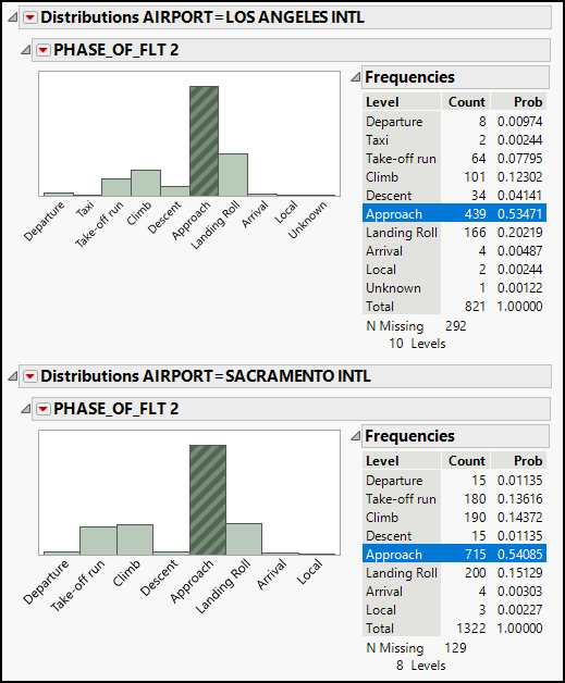
Figure 4.5 shows the results for two of the three airports. In general, the relative frequency of strikes is similar at both airports, though strikes during the Take-off run were more common in Sacramento than in Los Angeles, and just the opposite is true for strikes during the Landing Roll.
Based on Figure 4.4, we might have had the impression that none of the airports experienced half of the strikes during approach, despite the fact that just over 50% of all strikes occur during approach. We now see that for both L.A. and Sacramento, more than half of the strikes do occur during approach.
Why the difference between the two graphs? Missing observations. In L.A., we have Phase of Flight information about 821 strikes, but not for another 292 strikes. In other words, we have complete pairs of data for slightly less than three-quarters of all strikes (there were 821 + 292 = 1,113 strikes in L.A.). In contrast, the Phase of Flight was recorded for 91% of the strikes in Sacramento and 80% in San Francisco.
Another common way to display covariation in categorical variables is a crosstabulation (also known as a two-way table, a crosstab, a joint-frequency table, or a contingency table). JMP provides two different platforms that create crosstabs, and we will look at one of them here.
6. Select Analyze ► Fit Y by X. Select PHASE_OF_FLT 2 as Y, Response and Airport as X, Factor as shown in Figure 4.6.
Figure 4.6: Fit Y by X Contextual Platform
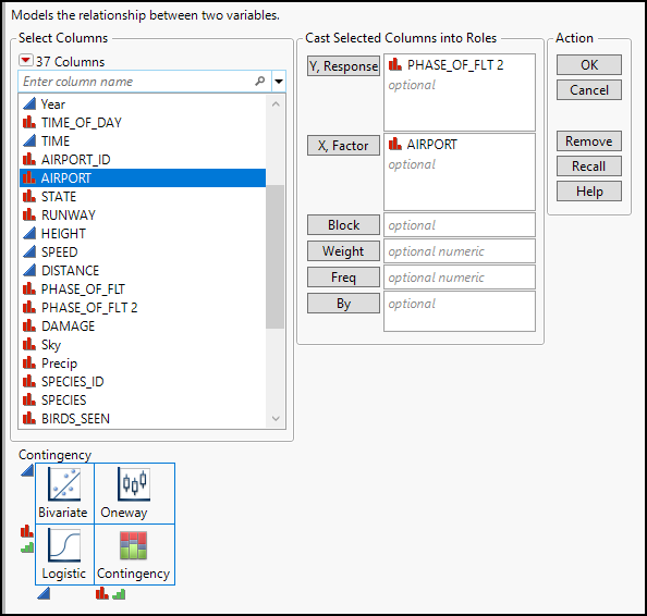
The Fit Y by X platform is contextual in the sense that JMP selects an appropriate bivariate analysis depending on the modeling types of the columns that you cast as Y and X. The four possibilities are shown in the lower left of the dialog box.
Figures 4.7 and 4.8 show the results of this analysis. We find a mosaic plot—essentially a visual crosstab—and a contingency table. In the mosaic plot, the vertical axis represents phase of flight, and the horizontal represents airports. The width and height of the rectangles in the mosaic are determined by the number of events in each category, and colors indicate the different phases of flight.
Figure 4.7: A Mosaic Plot of Wildlife Strikes at Three Airports
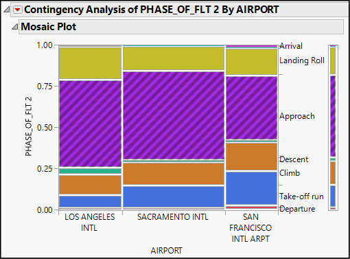
In this graph, the width of the vertical bars makes it clear that Sacramento had the greatest number of reported strikes that included phase of flight information, and San Francisco had the fewest. Though the data table includes 10 distinct phases of flight, we see labels for only the seven most commonly appearing in the data. Finally, the height of boxes is comparatively consistent across cities, indicating that strikes tend to occur during the same phases of flight at the three airports, with some minor variations.
The plot provides a clear visual impression, but if we want to dig into the specific numerical differences across regions, we turn to the Contingency Table (Figure 4.8). You might have heard tables like these called crosstabs or crosstabulations, or perhaps joint-frequency tables or two-way tables. All of these terms are synonymous.
Figure 4.8: A Crosstabulation of the Bird Strike Data
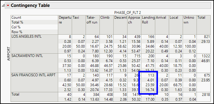
Across the top of this contingency table, we find the values of the PHASE_OF_FLT 2 column, and the rows correspond to the three airports. Each cell of the table contains four numbers representing the number of countries classified within the cell, as well as percentages computed for the full table, for the column, and for the row.
For example, look at the highlighted cell of the table in Figure 4.8. The numbers and their meanings are as follows:
|
113 |
113 reported incidents were strikes during the landing roll at San Francisco (SFO). |
|
4.01 |
4.01% of all 2,818 reported incidents fall into this cell (landing roll at SFO). |
|
23.59 |
23.59% of the 479 landing roll events occurred at SFO. |
|
16.74 |
16.74% of the 675 events at SFO occurred during landing roll. |
Describing Covariation: One Continuous, One Categorical Variable
We have just been treating phase of flight as a response variable, inquiring whether the prevalence of strikes during a particular phase varies depending on which airport was the site of the incident. With only minor differences, we found that strikes occur most often during the approach phase of the flight. We might wonder what it is about the approach phase that might account for the relatively high proportion of bird strikes—perhaps the altitude? The speed? With the data available to us here, we can begin to answer such questions.
To illustrate, let’s examine the distribution of flight speeds during the different flight phases. Consider that the observational units in our data table are incidents involving wildlife strikes. We are not observing all flights, and we aren’t observing incident-free flights (which constitute the vast majority of air travel). Hence, we can only describe aspects of those flights that did strike birds.
We have mentioned missing data before. This is another form of missing data, and it highlights another good habit of statistical thinking. For any set of data, it is wise to ask “what is not here?” The FAA Wildlife Strike database, by its nature, only contains data from flights that did have a bird strike. These flights are extraordinary in the context of all flights in the U.S.
1. Clear all row states (Rows menu).
2. Open the Graph Builder (Graph menu). Drag SPEED to the Y drop zone, and PHASE_OF_FLT 2 to the Group X drop zone at the top.
What do you see in your graph? As we might expect, the columns of jittered points tend to rise and fall with the familiar phases of flight. You might also notice that each of the speed distributions is asymmetric; there tend to be concentrations of many points at a relatively high or low speed. To visualize this more distinctly, we could make box plots or histograms of Speed by Phase of Flight. Instead, let’s learn a new type of graph:
3. In the menu bar at the top of Graph Builder, click the Contour icon (![]() ). This will create a violin plot, so called because some of the resulting shapes (see Figure 4.9) look a bit like violins.
). This will create a violin plot, so called because some of the resulting shapes (see Figure 4.9) look a bit like violins.
Figure 4.9: Violin Plot of Aircraft Speeds by Phase of Flight
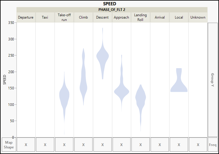
A violin plot shows the range of values for a variable; for example, those strikes that occurred during take-off run had recorded speeds between 50 and 200 mph. The narrow portion of the violin indicates very few takeoff strikes below 75 mph. The bulges in the violin indicate higher frequencies. It appears that strikes during takeoff are relatively common in the vicinity of 120 to 140 mph. Looking across all phases, one might say that except during descent, strikes are relatively frequent at speeds between approximately 120 and 160 mph regardless of flight phase.
For a more refined set of numerical summaries, do this:
4. Select Analyze ► Fit Y by X. Select SPEED as the Y column and PHASE_OF_FLT 2 as X and click OK.
5. For a numerical comparison, let’s look at some quantiles. In the Oneway Analysis report, click the red triangle and select Quantiles.
6. Below the graph should look like Figure 4.10.
Figure 4.10: Quantiles for Speed by Phase of Flight
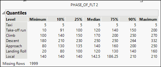
The table reports seven quantiles for each flight phase. We readily see strong similarities between speeds at the time of strikes for take-off run and landing roll, phases when the aircraft is on the ground. Quantiles during climb and approach are also comparable, but speeds during descent are uniformly higher than other phases.
Describing Covariation: Two Continuous Variables
To illustrate the standard bivariate methods for continuous data, we will now shift to a different set of data. In earlier chapters, we looked at variation in life expectancy around the world. We’ll now look at data related to variation in birth rates and the risks of childbirth in different nations as of 2017. We will rely on a data table with five continuous columns. Two of the columns measure the relative frequency of births in each country, and the other three measure risks to mothers and babies around birth. Initially, we will look at two of the variables: the columns labeled BirthRate and MortMaternal2016. A country’s annual birth rate is defined as the number of live births per 1,000 people in the country. The maternal mortality figure is the average number of mothers who die as a result of childbirth, per 100,000 births. At the time of this writing, the most current birth rate data was for 2017, but for maternal mortality, it was 2016.
As we did in the previous sections, let’s start by simply looking at the univariate summaries of these two variables.
1. Open the Birthrate 2017 data table.
2. Select Analyze ► Distribution. Cast BirthRate and MortMaternal in the Y role and click OK.
3. Within your BirthRate histogram, select different bars or groups of bars, and notice which bars are selected in the maternal mortality histogram. The results should look much like Figure 4.11.
Figure 4.11: Linked Histograms of Two Continuous Distributions
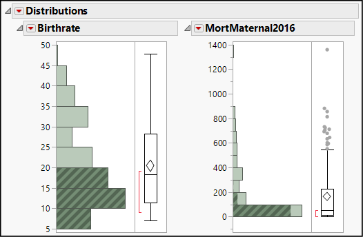
The general tendency is that countries with low birth rates also have low maternal mortality rates, but as one rate increases so does the other. We can see this tendency more directly in a scatterplot, an X-Y graph showing ordered pairs of values.
4. In the data table, press the Esc key to clear the de-select rows that you selected by clicking on histogram bars. Then choose Analyze ► Fit Y by X. Cast MortMaternal16 as Y and BirthRate as X and click OK.
Your results will look like those shown in Figure 4.12.
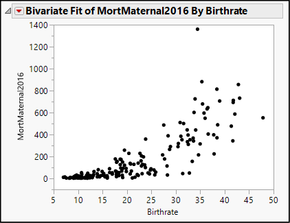
Figure 4.12: A Scatterplot
By now you also have had enough experience with Graph Builder to know that you can easily create a similar graph with that tool. You should feel free to explore data with Graph Builder.
This graph provides more information about the ways in which these two variables tend to vary together. First, it is very clear that these two variables do indeed vary together in a general pattern that curves upward from left to right; maternal mortality increases at an accelerating rate as the birth rate increases, though there are some countries that depart from the pattern. Many countries are concentrated in the lower left, with low birth rates and relatively low maternal mortality.
As we will learn in Chapters 15 through 19, there are powerful techniques available for building models of patterns like the one visible in Figure 4.12. At this early point in your studies, the curvature of the pattern presents some unwelcome complications. Figure 4.13 shows another pair of variables whose relationship is more linear. We will investigate this relationship and meet three common numerical summaries of such bivariate covariation.
5. Click the red triangle next to the word Bivariate in the current window and select Redo ► Relaunch Analysis.
6. Remove MortMaternal2016 from the Y, Response role and replace it with Fertil. This will produce a scatterplot (seen in modified fashion in Figure 4.13).
Earlier, we noted that birth rate counts the number of live births per 1,000 people in a country. Another measure of the frequency of births is the fertility rate, which is the mean number of children that would be born to a woman during her lifetime in each country.
When we look at this relationship in a scatterplot, we see that the points fall in a distinctive upward sloping pattern that is generally straight. We can also calculate three different numerical summaries to characterize the relationship. Each of the statistical measures compares the pattern of points to a perfectly straight line. The first summary is the equation of a straight line that follows the general trend of the points. (See Chapter 15 for a full explanation.) The second summary is a measure of the extent to which variation in X is associated with variation in Y, and the third summary measures the strength of the linear association between X and Y.
7. In the scatterplot of Fertility versus Birthrate, click the red triangle next to Bivariate Fit and select Fit Line.
8. Then click the red triangle again and select Histogram Borders.
Figure 4.13: Scatterplot with Histogram Borders and Line of Best Fit
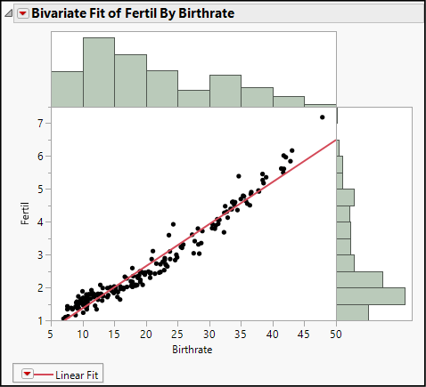
Now your results look like Figure 4.13. The consequence of these two customizations is that along the outside borders of the bivariate scatterplot, we see the univariate distributions of each of our two columns. Additionally, we see a red fitted line that approximates the upward pattern of the points.
Below the graph, we find the equation of that line:
Fertil = 0.0845109 + 0.1282129*BirthRate
The slope of this line describes how these two variables co-vary. If we imagine two groups of countries whose birth rates differ by one birth per 1,000 people, the group with the higher birth rate would average 0.128 more births per woman.
9. Below the linear fit equation, you will find the Summary of Fit table (not shown here). Locate the first statistic called Rsquare.
R square (r2) is a goodness-of-fit measure; for now, think of it as the proportion of variation in Y that is associated with X. If fertility were perfectly and completely determined as a linear function of birth rate, then R square would equal 1.00. In this instance, R square equals 0.958; approximately 96% of the cross-country variability in fertility rates is accounted for by differences in birth rates.
A third commonly used summary for bivariate continuous data is called correlation, which measures the strength of the linear association between the two variables. The coefficient of correlation, symbolized by the letter r, is the square root of r2 (if the slope of the best-fit line is negative, then r is –). As such, r always lies within the interval [–1, +1]. Values near the ends of the interval indicate strong correlations, and values near zero are weak correlations.
10. Select Analyze ► Multivariate Methods ► Multivariate. Cast both columns (BirthRate and Fertil) as Y and click OK. The upper part of your results will look like Figure 4.14.
Figure 4.14: A Correlation Matrix
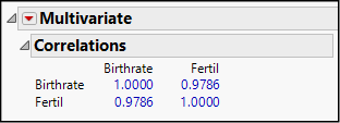
We find the correlation between birth rate and fertility rate to equal 0.9786, which is a very strong correlation. JMP uses a color scheme when reporting correlations. Strong positive values are in bright blue, and strong negative correlations are in bright red. Weaker values take on paler hues of blue and red, passing through gray near zero.
Scatter Plots for Very Large Data Tables
As the number of rows in a data table grows, we might encounter a common graphing problem called overplotting. When we attempt to plot many points in a fixed area, the points can become so densely packed that they overlap. At times, we may have multiple instances of the same X-Y pair, so that the graph gives the misimpression that there is a single point when there really might be several.
It is beyond the scope of this chapter to provide a full treatment of graphing large data sets, but this is an apt moment to look at a few strategies.
We have already encountered jittering in the univariate context. Jittering spreads points slightly to reveal when multiple points are at a single location. When the number of rows grows very large, jittering might not be enough.
To illustrate, we will consider the data in NHANES 2016, which contains detailed health information about nearly 10,000 people. We will use this data table extensively in our study of regression analysis. We first saw this data in Chapter 2. As part of the National Health and Nutrition Examination Survey, researchers measured the blood pressure of subjects multiple times. We will examine the covariation of systolic blood pressure (the “top” number) between the first and second readings for each person.
1. Open the data table NHANES 2016.
2. In Graph Builder, drag BPXSY1 to the X drop zone and BPXSY2 to the Y drop zone. This will treat the second reading as a function of the first reading.
Note that Graph Builder initially displays a point cloud and a smoother. It is obvious that we have many points that are densely packed in an elongated elliptical pattern. Try suppressing the display of points by clicking the left-most button in the menu bar. When there are so many points, one option for clarity is to simply show their trend without plotting every point. As we did earlier to create Figure 4.9, choosing the Contour option in the menu bar allows us to see the linear trend as well as regions that are most dense. The darkest contours here show the most common systolic pressure readings.
What if we want to see all 10,000 points more distinctly? Here are three options, among several others.
1. Click the left-most menu button to display all the points.
2. On the right side of the display, right-click over the legend ● BPXSY2
3. From the menu, select Marker to open a menu of marker shapes. Select an open circle or an X rather than a solid dot. After experimenting with a few shapes, return to the solid dot.
Depending on the density of the points, sometimes an open marker is preferable since it can show small spaces between nearby points, rather than having one occlude the other. In some graphs, reducing the size of each marker can achieve the same goal.
4. Again, right-click over the legend ● BPXSY2 and choose Marker Size to see the choices. The Preferred Size in this graph happens to be 3, Large. Try making them larger and smaller, noting how larger points tend to obscure one another in some parts of the graph. For the sake of the next step, leave the markers at size 5, XXL.
Similarly, rendering points as translucent helps with the overplotting problem. If we make the points partially transparent, then locations with multiple points will just appear darker in the graph. This effectively communicates which graph locations are most prevalent.
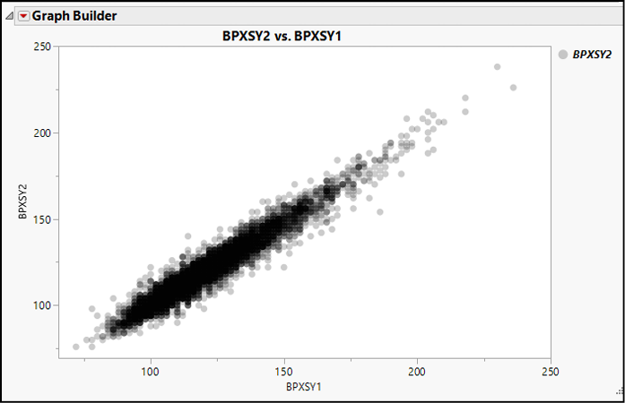
5. Right-click over the legend again and choose Transparency. By default, points are opaque with a transparency parameter of 1. Try setting transparency to 0.2, 0.5, and 0.8. Figure 4.15 shows this scatterplot with a transparency parameter of 0.2.
Figure 4.15: Using Transparency to Reveal Overplotting
More Informative Scatter Plots
This chapter has introduced ways to depict and summarize bivariate data, but sometimes we want or need to incorporate more than two variables into an analysis. We already know that with Graph Builder, we can color points to represent another variable, and we can wrap or overlay additional variables in a graph. We can use a By column in a Fit Y by X analysis to add a third factor into an investigation.
Another very useful visualization tool called a bubble plot provides a way to visualize as many as seven columns in one graph. This section provides a brief first look at bubble plots in JMP. We’ll use the tool further in Chapter 5.
Think of a bubble plot as a “scatterplot plus… .” In addition to the X-Y axes, the size and color of points can represent variables. Other variables can be used to interactively label points, and in cases where we have repeated measurements over time, the entire graph can be animated through time. Try this first exercise with the 2017 birth rate data:
1. Graph ► Bubble Plot. Cast Fertil as Y and Birthrate as X, just as before.
2. Next, cast Country as ID, Region as Coloring, and MortMaternal2016 as Sizes. Click OK.
3. In the lower left of the Bubble Plot window, find the slider control next to Bubble Size and slide it to the left until your graph looks like Figure 4.16.
Figure 4.16: Enhancing a Scatterplot by Using a Bubble Plot
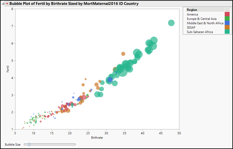
Compare this graph to Figure 4.13. The Y and X variables are the same, but this picture also conveys further descriptive generalizations; the highest birth and fertility rates are in sub-Saharan Africa, where maternal mortality rates are also the highest in the world. As you move your cursor around the graph, you will see hover labels identifying the points. You can also notice that countries with similar birth and fertility rates might have quite different maternal mortality rates (bubble sizes). Bubble plots pack a great deal of information into a compact, data-rich display.
Now that you have completed all of the activities in this chapter, use the concepts and techniques that you have learned to respond to these questions.
1. Scenario: We will continue to examine the World Development Indicators data in BirthRate 2017. We will broaden our analysis to work with other variables:
- Provider: Source of maternity leave benefits (public, private, or a combination of both)
- Fertil: Average number of births per woman during child-bearing years
- MortUnder5: Deaths of children under 5 years per 1,000 live births
- MortInfant: Deaths of infants per 1,000 live births
a. Create a mosaic plot and contingency table for the Provider and Region columns. Report on what you find.
b. Use appropriate methods to investigate how fertility rates vary across regions of the world. Report on what you find.
c. Create a scatterplot for MortUnder5 and MortInfant. Report the equation of the fitted line and the R-square value, and explain what you have found.
d. Is there any noteworthy pattern in the covariation of Provider and MatLeave90+? Explain what techniques you used, and what you found.
2. Scenario: How do prices of used cars differ, if at all, in different areas of the United States? How do the prices of used cars vary according to the mileage of the cars? Our data table Used Cars contains observational data about the listed prices of three popular compact car models in three different metropolitan areas in the U.S. The cities are Phoenix, AZ; Portland, OR; and Raleigh-Durham-Chapel Hill, NC. The car models are the Chrysler PT Cruiser Touring Edition, the Honda Civic EX, and the Toyota Corolla LE. The cars were all two years old at the time.
a. Create a scatterplot of price versus mileage. Report the equation of the fitted line, the R-square value, and the correlation coefficient, and explain what you have found.
b. Use the Graph Builder to see whether the relationship between price and mileage differs across different car models.
c. Describe the distribution of prices across the three cities in this sample.
d. Within this sample, are the different car models equally favored in the three different metropolitan areas? Discuss your analysis and explain what you have found.
3. Scenario: High blood pressure continues to be a leading health problem in the U.S. We have a data table (NHANES 2016) containing survey data from nearly 10,000 people in the U.S. in 2017. For this analysis, we will focus on only the following variables:
- RIAGENDR: Respondent’s gender
- RIDAGEYR: Respondent’s age in years
- RIDRETH1: Respondent’s racial or ethnic background
- BMXWT: Respondent’s weight in kilograms
- BPXPLS: Respondent’s resting pulse rate
- BPXSY1: Respondent’s systolic blood pressure (“top” number in BP)
- BPXD1: Respondent’s diastolic blood pressure (“bottom” number in BP)
a. Create a scatterplot of systolic blood pressure versus age. Within this sample, what tends to happen to blood pressure as people age?
b. Compute and report the correlation between systolic and diastolic blood pressure. What does this correlation tell you?
c. Use either a bubble plot to incorporate gender (Color) and pulse rate (Bubble Size) into the graph. Comment on what you see.
d. Compare the distribution of systolic blood pressure in males and females. Report on what you find.
e. Compare the distribution of systolic blood pressure by racial/ethnic background. Comment on any noteworthy differences that you find.
f. Create a scatterplot of systolic blood pressure and pulse rate. One might suspect that higher pulse rate is associated with higher blood pressure. Does the analysis bear out this suspicion?
4. Scenario: Despite well-documented health risks, tobacco is used widely throughout the world. The Tobacco data table provides information about the several variables for 133 different nations in 2005, including these:
- TobaccoUse: Prevalence of tobacco use (%) among adults 18 and older (both sexes)
- Female: Prevalence of tobacco use among females, 18 and older
- Male: Prevalence of tobacco use among males, 18 and older
- CVMort: Age-standardized mortality rate for cardiovascular diseases (per 100,000 population in 2002)
- CancerMort: Age-standardized mortality rate for cancers (per 100,000 population in 2002)
a. Compare the prevalence of tobacco use across the regions of the world, and comment on what you see.
b. Create a scatterplot of cardiovascular mortality versus prevalence of tobacco use (both sexes). Within this sample, describe the relationship, if any, between these two variables.
c. Create a scatterplot of cancer mortality versus prevalence of tobacco use (both sexes). Within this sample, describe the relationship, if any, between these two variables.
d. Compute and report the correlation between male and female tobacco use. What does this correlation tell you?
e. Create a bubble plot to modify your scatterplot from item c above to augment the display to incorporate region (color) and cardiovascular mortality (bubble size). Comment on what you find in the graph.
5. Scenario: Since 2003, the U.S. Bureau of Labor Statistics has been conducting the biennial American Time Use Survey. Census workers use telephone interviews and a complex sampling design to measure the amount of time people devote to various ordinary activities. We have some of the survey data in the data table called TimeUse. Our data table contains observations from more than 43,191 different respondents in 2003, 2007, and 2017. For these questions, use the Data Filter to select and include just the 2017 responses.
a. Create a crosstabulation of employment status by sex, and report on what you find.
b. Create a crosstabulation of full versus part-time employment status by gender, and report on what you find.
c. Compare the distribution of time spent sleeping across the employment categories. Report on what you find.
d. Now change the data filter to include all rows. Compare the distribution of time spent on personal email in 2003, 2007, and 2017. Comment on your findings.
6. Scenario: The data table Sleeping Animals contains information about the sizes, life spans, and sleeping habits of various mammal species. The last few columns are ordinal variables classifying the animals according to their comparative risks of being victimized by predators and the degree to which they sleep in the open rather than in enclosed spaces.
a. Create a crosstabulation of predation index by exposure index, and report on what you find.
b. Compare the distribution of hours of sleep across values of the danger index. Report on what you find.
c. Create a scatterplot of total sleep time and life span for these animals. What does the graph tell you?
d. Compute the correlation between total sleep time and life span for these animals. What does the correlation tell you?
7. Scenario: Let’s return to the data table FAA Bird Strikes CA. The FAA includes categorical variables pertaining to the number of birds struck, the size of the birds struck, and the general weather conditions.
a. Create a crosstabulation of number of birds struck versus sky conditions (Sky), and report on what you find.
b. Create a crosstabulation of number of birds struck versus the precipitation conditions (Precip), and report on what you find.
c. Investigate the relationship between the number of birds struck and the speed of the aircraft. Write a sentence to describe that relationship.
d. Investigate the relationship between the number of birds struck and the height of the aircraft. Write a sentence to describe that relationship.
8. Scenario: Every ten years, the United States conducts a census of the population, gathering considerable data about the nation and its residents. The data table called USA Counties contains demographic, economic, commercial, educational, and other data about each of the 3,143 counties in the United States as of 2010.
a. Create a scatterplot of median household income (Y) versus percent of the population with a bachelor’s degree. Comment on what you see.
b. Compute and report the line of best fit for these data. Use that line to estimate the median household income in counties with 25% of the population holding bachelor’s degrees.
c. Create and report on a scatterplot between the percentage of households where a foreign language is spoken in the home (foreign_spoken_at_home) and the percentage of households with a foreign-born member (foreign_born). How do you explain the distinctive pattern in the graph?
d. Compute and explain the correlation coefficient for the two variables in item c above.
e. Estimate the line of best fit using the population as determined by the 2010 US Census as Y and the 2000 population count as X. Think about the slope of this line. What does it tell us about what happened to the average of US counties’ populations between 2000 and 2010?
f. The point representing Cook County, Illinois, is distinctive in that it lies below the red estimated line (2000 population was 5,194,675). According to this fitted line, what was unusual about Cook County in comparison to other counties of the United States?