
Chapter 13: Two-Sample Inference for a Continuous Variable
Using JMP to Compare Two Means
Assuming Normal Distributions or CLT
Using Sampling Weights (Optional Section)
Equal Versus Unequal Variances
Dealing with Non-Normal Distributions
Using JMP to Compare Two Variances
At the end of the prior chapter, we studied the matched pairs design to make inferences about the mean of differences within a population. In this chapter, we take up the comparison of samples drawn independently from two different populations and learn to estimate the differences between population means and variances. The procedures discussed here assume that samples are randomized (and therefore representative) and are comparatively small subsets of their respective populations.
We will first focus on the centers of the two populations and assume that measurements are independent both within and across samples. As we did in the last chapter, we begin with cases in which the populations are either approximately normal or in which the Central Limit Theorem applies. Then, we will see a nonparametric (also known as distribution-free) approach for non-normal data. Finally, we will learn to compare the spread of two distributions as measured by the variance.
Using JMP to Compare Two Means
We have used the NHANES 2016 data to illustrate many statistical concepts, and we will return to it again now. Recall that the National Health and Nutrition Examination Survey is a biennial cross-sectional sample conducted by the U.S. Centers for Disease Control. Within this large data table there are several measurements typically taken during a routine physical exam. For some of these measurements, we expect to find differences between male and female subjects. Men tend to be taller and heavier than women, for example. But are their pulse rates different? In our first illustration, we will estimate the difference (if any) between the resting pulse rates of adult women and men.
Assuming Normal Distributions or CLT
1. Open the NHANES 2016 data table.
The subjects in the NHANES 2016 data table range in age from infants up. Our first step is to exclude subjects under the age of 18 years. We will use the Data Filter to select just the adults.
2. Select Rows ► Data Filter. As shown in the left side of Figure 13.1, choose the RIDAGEYR column and click Add.
Figure 13.1: Using the Data Filter to Restrict Analysis to Adults
|
|
|
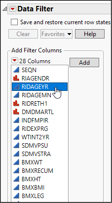
3. In the filter, check the boxes as shown and edit the minimum age to equal 18.
Before performing any inferential analysis, let’s look at the pulse rate data, separating the observations for females and males.
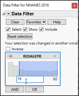
4. Select Analyze ► Distribution. Cast BPXPLS (pulse rate) into Y and RIAGENDR into By.
5. In the Distribution report, click the red triangle next to Distributions, and select Stack to create the report shown in Figure 13.2.
Figure 13.2: Distribution of Pulse Rate by Gender
A quick glance suggests that each distribution is reasonably symmetric with a central peak and similar measures of dispersion. Given that fact as well as the large size of the samples, we can conclude that we are on solid ground using a t test. As in the one-sample case, the t test is reliable when the underlying population is approximately normal or when the samples are large enough for the Central Limit Theorem to apply. We have very large samples, so we will rely on the CLT to proceed with the analysis.
Conceptually, we are about to investigate a statistical model. The model says “gender may account for some of the variability in individual pulse rates.” The conventional language that we use is to say that we are “fitting” a model for Y as a function of X. As you will see in the Fit Y by X dialog box, we will cast pulse rate as a response to a varying factor, gender.
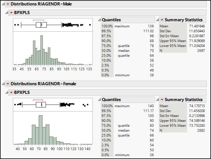
6. Select Analyze ► Fit Y by X. Select BPSXPLS as Y, Response and RIAGENDR as X, Factor, and click OK.
7. Move your cursor over the graph and right-click to open a menu. Choose Marker Size ► 0, Dot. With more than 2,000 observations for each gender, the default dot size makes it difficult to see the individual points.
8. Click the red triangle next to Oneway Analysis, and select Display Options ► Points Jittered. This randomly spaces out the points horizontally for each group, adding further resolution to the image.
9. Click the same red triangle again and select Display Options ► Box Plots. When you have done this, your report looks like Figure 13.3.
Figure 13.3: Bivariate Comparison of Pulse Rates
In this graph, we see side-by-side box plots of the observations. The box plots illustrate the symmetry of the two distributions and suggest that they have similar centers and dispersion. Though this graph re-displays some of the information from Figure 13.2, here we get a clearer sense of just how the points are distributed.
The Fit Y by X platform allows us to test whether there is a statistically significant difference between the mean pulse rates of men and women based on these two large subsamples, and to estimate the magnitude of the difference (if any).
10. Click the red triangle once more, and select t Test. This produces the results shown in Figure 13.4.
You might have noticed that, unlike the one-sample t test, this command gives us no option to specify a hypothesized difference of means. Usually, the two-sample t test has as its default the null hypothesis of no difference. In other words, the default setting is that the difference in means equals 0. This version of the two-sample t test assumes that the variances of the two populations are unequal; we will discuss that assumption shortly.
Figure 13.4: Results of a Bivariate t Test
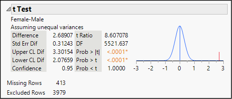
In the results panel, we see that there was a difference of 2.69 beats per minute between the females and males in the sample. We also find the 95% confidence interval for the difference in population means. Based on these two samples of women and men, we estimate that in the population at large, women’s pulse rates are 2.08 to 3.30 beats per minute higher than men’s.
We also see a t-distribution centered at 0 and a red line marking the observed difference within the sample. The observed difference of nearly 2.7 beats is more than 8.61 standard errors from the center—something that is virtually impossible by chance alone. Whether or not you expected to find a difference, these samples lead us to conclude that there is one.
Using Sampling Weights (Optional Section)
The NHANES 2016 data comes from a complex sample, and the data table includes sampling weights. To conduct inferential analysis properly with surveys like NHANES, we should apply the post-stratification weights. The weights do alter the estimated means and standard errors and therefore lead to slightly different conclusions. We interpret weighted results exactly as described above, and the software makes it very easy to apply the weights.
1. Click the red triangle next to Oneway Analysis and choose Redo ► Relaunch. This re-opens the launch dialog box with BPXPLS cast as Y and RIAGENDR as X. Add WTINT2YR as Weight.
All other instructions and interpretations are as described above. Notice that the t test results have changed. While still quite significant, the estimated gender difference in pulse rate is not quite as large as we previously thought. Applying the sampling weights provides more accuracy, but is a topic that is typically excluded from an introductory course.
Equal Versus Unequal Variances
The t test procedure we just performed presumed that the variance in pulse rates for women and men are unequal and estimated the variance and standard deviation separately based on the two samples. That is a conservative and reasonable thing to do.
If we can assume that the populations not only share a common normal shape (or that the Central Limit Theorem applies because both samples are large) but also share a common degree of spread, we can combine the data from the two samples to estimate that shared variance. With smaller samples, there is some gain in efficiency if we can combine, or pool, the data to estimate the unknown population variances. Later in this chapter, we will see a way to test whether the variances are equal or not. At this point, having noted that the samples seem to have similar spread, let’s see how the pooled-variance version of this test operates.
2. Return to the first Oneway Analysis report. Click the red triangle, and select Means/Anova/Pooled t. This produces the results shown in Figure 13.5.
Figure 13.5: The Pooled Variance t Test
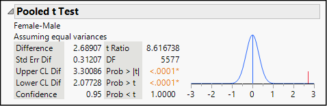
This command produces several new items in our report, all within a panel labeled Oneway Anova. We will devote all of Chapter 14 to ANOVA (Analysis of Variance) and will not say more about it here. Locate the heading Pooled t Test and confirm that the report includes the phrase Assuming equal variances. We read and interpret these results exactly as we did in the unequal variance test.
Because the two sample variances are very similar and the samples are so large, these results are extremely close to the earlier illustration. The estimated pooled standard error (Std Err Dif) is just slightly smaller, so the resulting confidence interval is a bit narrower in this procedure.
Dealing with Non-Normal Distributions
Let’s look again at the pipeline safety data, confining our attention to just two states of the United States—Texas and Oklahoma, the states with the largest number of incidents in this data table. Moreover, to illustrate the challenge of non-normal data from samples too small to rely on the Central Limit theorem, we will also analyze only those disruptions that occurred in 2018. We will compare the cost of gas released, assuming that disruptions and their repairs are independent in the two regions over time.
1. Open the Pipeline Safety data table.
2. Use the Data Filter to show and include only those leaks occurring in Oklahoma or Texas (Op_State column; state abbreviations are OK and TX) AND select, show, and include rows where IYEAR = 2018.
3. Select Analyze ► Distribution. Select EST_COST_GAS_RELEASED as Y, Op_State as By, and click OK. This creates two histograms, one for each region.
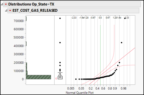
According to the reported quantiles and summary statistics, the observed incidents in Oklahoma had a median cost of $11,600 and a mean of $12,495. In contrast, the median was $17,485.50 and the mean was $44,625.57 in Texas. This is apparently a large difference, but is it statistically significant? We have only 19 observations from Oklahoma and 62 from Texas. Before running a t test as before, we should check for normality in these two small samples. The histograms are strongly skewed to the right, but let’s also look at a normal quantile plot.
4. Hold the Ctrl key, click the red triangle next to Distributions, and check Normal Quantile Plot; the Texas results are shown in Figure 13.6.
Figure 13.6: Normal Quantile Plot for a Strongly Skewed Distribution
We have two skewed distributions with relatively small samples. We cannot invoke the Central Limit Theorem as needed to trust the t test, but we do have nonparametric options available. It is beyond the scope of most introductory courses to treat nonparametric alternatives in depth, but we will illustrate one of them here because it is commonly used. The null hypothesis of the test is that the two distributions of EST_COST_GAS_RELEASED are centered at the same dollar value.
5. Select Analyze ► Fit Y by X. The Y, Response column is EST_COST_GAS_RELEASED and the X, Factor column is Op_State. Click OK.
6. Click the red triangle next to Oneway Analysis and select Display Options ► Box Plots. This provides an easy visual comparison of the two distributions.
7. Click the red triangle again, and select Nonparametric ► Wilcoxon Test. This generates the report shown in Figure 13.7.
Figure 13.7: Results of a Two-Sample Wilcoxon Test
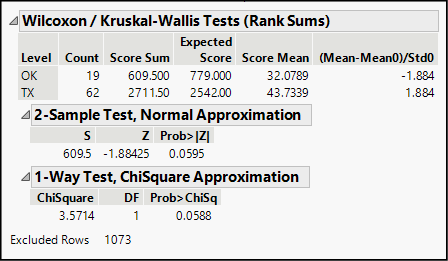
When we have two samples, as we do here, JMP conducts a Wilcoxon test, which is the equivalent of another test known as the Mann-Whitney U Test. With more than two samples, JMP performs and reports a Kruskal-Wallis Test (as we will see in Chapter 14). The common approach in these tests is that they combine all observations and rank them. They then sum up the rankings for each group (region, in this case) and find the mean ranking. If the two groups are centered at the same value, then the mean ranks should be very close. If one group were centered at a very different point, the mean ranks would differ by quite a lot.
Naturally, the key question is, “how much of a difference is considered significant?” Suffice it to say that JMP uses two conventional methods to estimate a P-value for the observed difference in mean ranks. Both methods use approximations to a standard distribution; the first test relies on a Normal model, and the second on a Chi-Square model. The two P-values appear in the lower portion of Figure 13.7 and are quite similar. The alpha risk—the risk of a Type I error—is very near the conventional 5% level. Depending on the context of the decision, a decision-maker may or may not find the observed difference statistically significant. In a published article, an author might say that the difference is significant at the 0.10 level but not at the 0.05 level.
Using JMP to Compare Two Variances
In our earlier discussion of the t test, we noted that there are two versions of the test, corresponding to the conditions in which the samples share the same variance or have different variances. Both in the t tests and in techniques we will see later, we might need to decide whether two or more groups have equal or unequal variances before we choose a statistical procedure. The Fit Y by X platform in JMP includes a command that facilitates the judgment.
Let’s shift back to the NHANES 2016 data and consider the Body Mass Index for the adult men and women (ages 18 and older) in the samples. BMI is a measure of body fat as a percentage of total weight. A lean person has lower BMI than an overweight person. We will test the hypothesis that adult women and men in the US have the same mean BMI, and before choosing a test, we will compare the variances of the two populations.
1. Return to the NHANES 2016 data table. Make sure that you are still showing and including respondents 18 years of age and older.
2. Select Analyze ► Fit Y by X. Our Y column is BMXBMI and our X column is RIAGENDR.1 Click OK.
3. Click the red triangle next to Oneway Analysis and select UnEqual Variances. This opens the panel shown in Figure 13.8.
Figure 13.8: Testing for Equal Variances
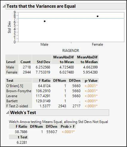
We find a simple graph comparing the sample standard deviations (s) of the two groups, with the numerical summaries below it. For the women, s = 7.75, and for the men, s = 6.25. Because the variance is the square of the standard deviation, we can determine that the sample variances are approximately 60.1 and 39.1, respectively. Based on these sample values, should we conclude that the population variances are the same or different?
JMP performs five different tests for the equality, or homogeneity, of variances. Although they all lead to the same conclusion in this example, that is not always the case. For two-sample comparisons, the most commonly used tests are probably Levene’s test and the F test two-sided. The null hypothesis is that the variance of all groups is equal, and the alternative hypothesis is that variances are unequal.
In this example, the P-values fall well below the conventional significance level of 0.05. That is, there is enough evidence to reject the null assumption of equal variances, so we can conclude that this set of data should be analyzed with an unequal variance t test. You can perform the test as one of the Application exercises at the end of the chapter.
Now that you have completed all of the activities in this chapter, use the concepts and techniques that you have learned to respond to these questions. Be sure to examine the data to check the conditions for inference, and explain which technique you used, why you chose it, and what you conclude.
1. Scenario: Let’s continue analyzing the data for adults in the NHANES 2016 data table. For each of the following columns, estimate the difference between the male and female respondents using a 95% confidence level.
a. What is the estimated difference in Body Mass Index (BMI)?
b. What is the estimated difference in systolic blood pressure?
c. What is the estimated difference in diastolic blood pressure?
d. What is the estimated difference in waist circumference?
2. Scenario: We will continue our analysis of the pipeline disruption data in Oklahoma and Texas. The column EST_COST_PROP_DAMAGE contains the dollar value of property damage as a consequence of the disruption.
a. Report and interpret a 95% confidence interval for the difference in mean property value costs of a pipeline disruption.
b. Test the hypothesis that there is no difference in the mean property damage costs between the two states.
3. Scenario: Go back to the full Pipeline Safety data table. Clear row states to show and include all states and years. We will compare the age of pipelines in locations controlled by the operator and those that are public rights of way.
a. Use the Distribution platform to inspect the distributions of YRS_IN_PLACE by LOCATION_TYPE. Write a sentence comparing the two distributions. Does your inspection of the distributions give the impression that they are similar or different?
b. Estimate the difference in years in place for lines on Operator-Controlled Property versus Pipeline Right-of-Way. Assume for the moment that utility companies can more easily perform maintenance on property that they control. Interpret your findings in light of this assumption.
c. Test the hypothesis that the variances are equal in comparing pipeline for leaks versus ruptures. Explain your conclusion.
4. Scenario: Parkinson’s disease (PD) is a neurological disorder affecting millions of older adults around the world. Among the common symptoms are tremors, loss of balance, and difficulty in initiating movement. Other symptoms include vocal impairment. We have a data table, Parkinsons (Little, McSharry, Hunter, & Ramig, 2008), containing a number of vocal measurements from a sample of 32 patients, 24 of whom have PD.
Vocal measurement usually involves having the patient read a standard paragraph, or sustain a vowel sound, or do both. Two common measurements of a patient’s voice refer to the wave form of sound: technicians note variation in the amplitude (volume) and frequency (pitch) of the voice. In this scenario, we will focus on just three measurements.
◦ MDVP:F0(Hz): Vocal fundamental frequency (baseline measure of pitch)
◦ MDVP:Jitter(Abs): Jitter refers to variation in pitch
◦ MDVP:Shimmer(db): Shimmer refers to variation in volume
a. Examine the distributions of these three columns, distinguishing between patients with and without PD. Do these data meet the conditions for running and interpreting a two-sample t test? Explain your thinking.
b. Use an appropriate technique to decide whether PD and non-PD patients have significantly different baseline pitch measurements.
c. Use an appropriate technique to decide whether PD and non-PD patients have significantly different jitter measurements.
d. Use an appropriate technique to decide whether PD and non-PD patients have significantly different shimmer measurements.
5. Scenario: The data table Airline Delays contains a sample of flights for four airlines destined for three busy airports. Our goal is to analyze the delay times, expressed in minutes, and compare two of the airports. First, use the Data Filter to show and include only those flights destined for Atlanta and Chicago.
a. Assume this is an SRS of many flights by the selected carriers and airports over a long period of time. Is the variance of delay the same for both airports?
b. What can you conclude about the difference in mean delays for these two airlines?
6. Scenario: Let’s look again at the TimeUse data. For each of the following questions, evaluate the extent to which conditions for inference have been met, and then report on what you find when you use an appropriate technique.
a. Estimate the mean difference in the amount of time men and women spent sleeping in 2017.
b. Estimate the mean difference in time that individuals devoted to email in 2007 versus 2017.
c. What can you conclude about the difference in the mean amount of time spent by women and men socializing on a given day across all years?
7. Scenario: This question looks at the NC Births data. For each of the following questions, evaluate the extent to which conditions for inference have been met, and then report on what you find when you use an appropriate technique.
a. Do babies born to mothers who smoke weigh less than those born to non-smokers?
b. Estimate the mean weight gain among pregnant smokers and non-smokers.
c. Do smokers and non-smokers deliver their babies after the same number of weeks, on average?
Endnotes
1 If you want to use sampling weights in the analysis, use the weight column WTINT2YR.