
Chapter 2: Data Sources and Structures
Populations, Processes, and Samples
Representativeness and Sampling
Cross-Sectional and Time Series Sampling
Study Design: Experimentation, Observation, and Surveying
Raw Case Data and Summary Data
This chapter is about data. More specifically, it is about how we make choices when we gather or generate data for analysis in a statistical investigation, and how we store that data in JMP files for further analysis. This chapter introduces some data storage concepts that are further developed in Appendix B. How and where we gather data are the foundation for what types of conclusions and decisions we can draw. After reading this chapter, you should have a solid foundation to build upon.
Populations, Processes, and Samples
We analyze data because we want to understand something about variation within a population—a collection of people or objects or phenomena that we are interested in. Sometimes we are more interested in the variability of a process—an ongoing natural or artificial activity (like the occurrences of earthquakes or fluctuating stock prices). We identify one or more variables of interest and either count or measure them.
In most cases, it is impossible or impractical to gather data from every single individual within a population or every instance from an ongoing process. Marine biologists who study communication among dolphins cannot possibly measure every living dolphin. Manufacturers wanting to know how quickly a building material degrades in the outdoors cannot destroy 100% of their products through testing or they will have nothing left to sell. Thanks to huge databases and powerful software, financial analysts interested in future performance of a stock can analyze every single past trade for that stock, but they cannot analyze trades that have not yet occurred.
Instead, we typically analyze a sample of individuals selected from a population or process. Ideally, we choose the individuals in such a way that we can have some confidence that they are a “second-best” substitute or stand-in for the entire population or ongoing process. In later chapters, we will devote considerable attention to the adjustments that we can make before generalizing sample-based conclusions to a larger population.
As we begin to learn about data analysis, it is important to be clear about the roles and relationship of a population and a sample. In many statistical studies, the situation is as follows (this example refers to a population, but the same applies to a process):
● We are interested in the variation of one or more attributes of a population. Depending on the scenario, we may wish to anticipate the variation, influence it, or just understand it better.
● Within the context of the study, the population consists of individual observational units, or cases. We cannot gather data from every single individual within the population.
● Hence, we choose some individuals from the population and observe them to generalize about the entire population.
We gather and analyze data from the sample of individuals instead of doing so for the whole population. The individuals within the sample are not the group that we are ultimately interested in knowing about. We really want to learn about the variability within the population. When we use a sample instead of a population, we run some risk that the sample will misrepresent the population—and that risk is at the center of statistical reasoning.
Depending on just what we want to learn about a process or population, we also concern ourselves with the method by which we generate and gather data. Do we want to characterize or describe the extent of temperature variation that occurs in one part of the world? Or do we want to understand how patients with a disease respond to a specific dosage of a medication? Or do we want to predict which incentives are most likely to induce consumers to buy a product?
There are two types of generalizations that we might eventually want to be able to make, and in practice, statisticians rely on randomization in data generation as the logical path to generalization. If we want to use sample data to characterize patterns of variation in an entire population or process, it is valuable to select sample cases using a probability-based or random process. If we ultimately want to draw definitive conclusions about how variation in one variable is caused or influenced by another, then it is essential to randomly control or assign values of the suspected causal variable to individuals within the sample.
Therefore, the design strategy in sampling is terrifically important in the practical analysis of data. We also want to think about the time frame for sampling. If we are interested in the current state of a population, we should select a cross-section of individuals at one time. On the other hand, if we want to see how a process unfolds over time, we should select a time series sample by observing the same individual repeatedly at specific intervals. Some samples (often referred to as panel data) consist of a list of individuals observed repeatedly at a regular interval.
Representativeness and Sampling
If we plan to draw general conclusions about a population or process from one sample, it’s important that we can reasonably expect the sample to represent the population. Whenever we rely on sample information, we run the risk that the sample could misrepresent the population. (In general, we call this sampling error.) Statisticians have several standard methods for choosing a sample. No one method can guarantee that a single sample accurately represents the population, but some methods carry smaller risks of sampling error than others. What’s more, some methods have predictable risks of sampling error, while others do not. As you will see later in the book, if we can predict the extent and nature of the risk, then we can generalize from a sample; if we cannot, we sacrifice our ability to generalize. JMP can accommodate different methods of representative sampling, both by helping us to select such samples and by taking the sampling method into account when analyzing data. At this point, we focus on understanding different approaches to sampling by examining data tables that originated from different designs. We will also take a first look at using JMP to select representative samples. In Chapters 8 and 21, we will revisit the subject more deeply.
Simple Random Sampling
The logical starting point for a discussion of representative sampling is the simple random sample (SRS). Imagine a population consisting of N elements (for example, a lake with N = 1,437,652 fish), from which we want to take an SRS of n = 200 fish. With a little thought, we recognize that there are many different 200-fish samples that we might draw from the lake. If we use a sampling method that ensures that all 200-fish samples have the same chance of being chosen, then any sample we take with that method is an SRS. Essentially, we depend on the probabilities involved in random sampling to produce a representative sample.
Simple random sampling requires that we have a sampling frame, or a list of all members of a population. The sampling frame could be a list of students in a university, firms in an industry, or members of an organization. To illustrate, we will start with a list of the countries in the world and see one way to select an SRS. For the sake of this example, suppose we want to draw a simple random sample of 20 countries for in-depth research.
There are several ways to select and isolate a simple random sample drawn from a JMP data table. In this illustration, we will first randomly select 20 rows, and then proceed to move them into a new data table. This is not the most efficient method, but it emphasizes the idea of random selection, and it introduces two useful commands.
In this chapter, we will work with several data tables. As such, this is an opportunity to introduce JMP Projects. A project keeps track of data and report files together.
1. First, we will create a Project to store the work that we are about to do. File ► New ► Project. A blank project window opens. (See Figure 2.1.)
Figure 2.1: A Project Window
2. File ► Open. Select the data table called World Nations. This table lists the countries in the world as of 2017, as identified by the United Nations and the World Bank. Notice that the data table opens within the project window, and the Windows List in the upper left contains World Nations.
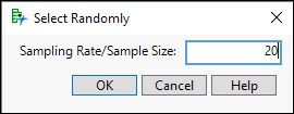
3. Select Rows ► Row Selection ► Select Randomly…. A small dialog box opens (Figure 2.2) asking either for a sampling rate or a sample size. If you enter a value between 0 and 1, JMP understands it as a rate. A number large than 1 is interpreted as a sample size, n. Enter 20 into the dialog box and click OK.
Figure 2.2: Specifying a Simple Random Sample Size of 20
JMP randomly selects 20 of the 215 rows in this table. When you look at the Rows panel in the Data Table window, you will see that 20 rows have been selected. As you scroll down the list of countries, you will see that 20 selected rows are highlighted. If you repeat Step 2, a different list of 20 rows will be highlighted because the selection process is random. If you compare notes with others in your class, you should discover that their samples comprise different countries. With the list of 20 countries now chosen, let’s create a new data table containing just the SRS of 20 countries.
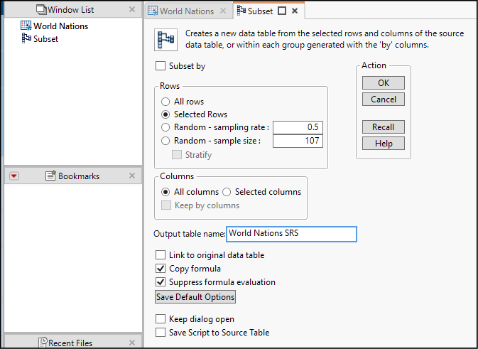
4. Select Tables ► Subset. This versatile dialog box (see Figure 2.3) enables us to build a table using the just-selected rows, or to randomly sample directly. Note that the dialog box opens in a fresh tab within the Project, and as an item in the Window List.
5. As shown in the figure, choose Selected Rows and then change the Output table name to World Nations SRS. Then click OK.
Figure 2.3: Creating a Subset of Selected Rows
In the upper left corner of the data table window, there is a green arrow with the label Source. JMP inserts the JSL script that created the subset. Readers wishing to learn more about writing JMP scripts should right-click the green arrow, choose Edit, and see what a JSL script looks like.
Before moving to the next example, let’s save the Project. Before saving a project, all documents within the project must be saved individually. We just created a new data table; save it now.
6. File ► Save. The default name is World Nations SRS, which is fine. Place it in a folder of your choice.
7. File ► Save Project. Choose a location and name this project Chap_02. Then, click OK. Among your Recent Files list, you will now find Chap_02.jmpprj.
Other Types of Random Sampling
As noted previously, simple random sampling requires that we can identify and access all N elements within a population. Sometimes this is not practical, and there are several alternative strategies available. It is well beyond the scope of this chapter to discuss these strategies at length, but Chapter 8 provides basic coverage of some of these approaches.
Non-Random Sampling
This book is about practical data analysis, and in practice, many data tables contain data that were not generated by anything like a random sampling process. Most data collected within businesses and nonprofit organizations come from the normal operations of the organization rather than from a carefully constructed process of sampling. The data generated by “Internet of Things” devices, for example, are decidedly non-random. We can summarize and describe the data within a non-random sample but should be very cautious about the temptation to generalize from such samples. Whether we are conducting the analysis or reading about it, we always want to ask whether a given sample is likely to misrepresent the population or process from which it came. Voluntary response surveys, for example, are very likely to mislead us if only highly motivated individuals respond. On the other hand, if we watch the variation in stock prices during an uneventful period in the stock markets, we might reasonably expect that the sample could represent the process of stock market transactions.
Big Data
You might have heard or read about “Big Data”—high volume raw data generated by numerous electronic technologies like cell phones, supermarket scanners, radio-frequency identification (RFID) chips, or other automated devices. The world-spanning, continuous stream of data carries huge potential for the future of data analytics and presents many ethical, technical, and economic challenges. In general, data generated in this way are not random in the conventional sense and don’t neatly fit into the traditional classifications of an introductory statistics course. Big data can include photographic images, video, or sound recordings that don’t easily occupy columns and rows in a data table. Furthermore, streaming data is neither cross-sectional nor time series in the usual sense.
Cross-Sectional and Time Series Sampling
When the research concerns a population, the sampling approach is often cross-sectional, which is to say the researchers select individuals from the population at one period of time. Again, the individuals can be people, animals, firms, cells, plants, manufactured goods, or anything of interest to the researchers.
When the research concerns a process, the sampling approach is more likely to be time series or longitudinal, whereby a single individual is repeatedly measured at regular time intervals. A great deal of business and economic data is longitudinal. For example, companies and governmental agencies track and report monthly sales, quarterly earnings, or annual employment. The major distinction between time series data and streaming data is whether observations occur according to a pre-determined schedule or whether they are event-driven (for example, when a customer places a cell phone call).
Panel studies combine cross-sectional and time series approaches. In a panel study, researchers repeatedly gather data about the same group of individuals. Some long-term public health studies follow panels of individuals for many years; some marketing researchers use consumer panels to monitor changes in taste and consumer preferences.
Study Design: Experimentation, Observation, and Surveying
If the goal of a study is to demonstrate a cause-and-effect relationship, then the ideal approach is a designed experiment. The hallmark features of an experiment are that the investigator controls and manipulates the values of one or more variables, randomly assigns treatments to observational units, and then observes changes in the response variable. For example, engineers in the concrete industry might want to know how varying the amount of different additives affects the strength of the concrete. A research team would plan an experiment in which they would systematically vary specific additives and conditions, then measure the strength of the resulting batch of concrete.
Similarly, consider a large retail company that has a “customer loyalty” program, offering discounts to its regular customers who present their bar-coded key tags at the check-out counter. Suppose the firm wants to nudge customers to return to their stores more frequently and generates discount coupons that can be redeemed if the customer visits the store again within so many days. The marketing analysts in the company could design an experiment in which they vary the size of the discount and the expiration date of the offer, issue the different coupons to randomly chosen customers, and then see when customers return.
In an experimental design, the causal variables are called factors, and the outcome variable is called the response variable. As an illustration of a data table containing experimental data, open the data table called Concrete. Professor I-Cheng Yeh of Chung-Hua University in Taiwan measured the compressive strength of concrete prepared with varying formulations of seven different component materials. Compressive strength is the amount of force per unit of area, measured here in megapascals that the concrete can withstand before failing. Think of the concrete foundation walls of a building; they need to be able to support the mass of the building without collapsing. The purpose of the experiment was to develop an optimal mixture to maximize compressive strength.
1. Select File ► Open. Choose Concrete and click OK.
Figure 2.4: The Concrete Data Table (Within Project)
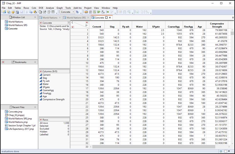
The first seven columns in the data table in Figure 2.4 represent factor variables. Professor Yeh selected specific quantities of the seven component materials and then tested the compressive strength as the concrete aged. The eighth column, Age, shows the number of days elapsed since the concrete was formulated, and the ninth column is the response variable, Compressive Strength. In the course of his experiments, Professor Yeh repeatedly tested different formulations, measuring compressive strength after varying numbers of days. To see the structure of the data, let’s look more closely at the two columns.
8. Choose Analyze ► Distribution.
9. As shown in Figure 2.5, select the Cement and Age columns and click OK.
Figure 2.5: The Distribution Dialog Box
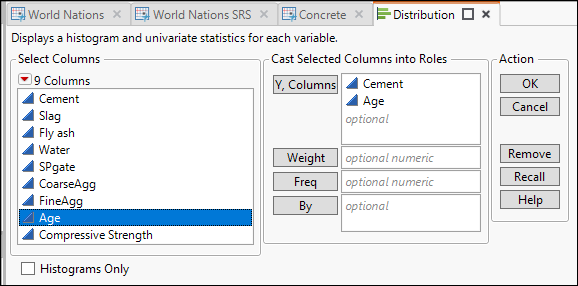
The Distribution platform generates two graphs and several statistics. We will study these in detail in Chapter 3. For now, you just need to know that the graphs, called histograms, display the variation within the two data columns. The lengths of the bars indicate the number of rows corresponding to each value. For example, there are many rows with concrete mixtures containing about 150 kg of cement, and very few with 100 kg.
10. Move your cursor over the Cement histogram and click the bar corresponding to values just below 400 kg of cement.
When you click that bar, the entire bar darkens, indicating that the rows corresponding to mixtures with that quantity (380 kg of cement, it turns out) are selected. Additionally, small portions of several bars in the Age histogram are also darkened, representing the same rows.
11. To see the relationships between a histogram bar, the data table, and the other histogram, we want to make the Distribution Report and Data Table visible at the same time. Move your cursor over the tab labeled Concrete – Distribution of Cement, Age. Click and drag downward; release the button over the Dock Above zone. The windows should look like Figure 2.6. Save your project once more.
Figure 2.6: Select Rows by Selecting One Bar in a Graph
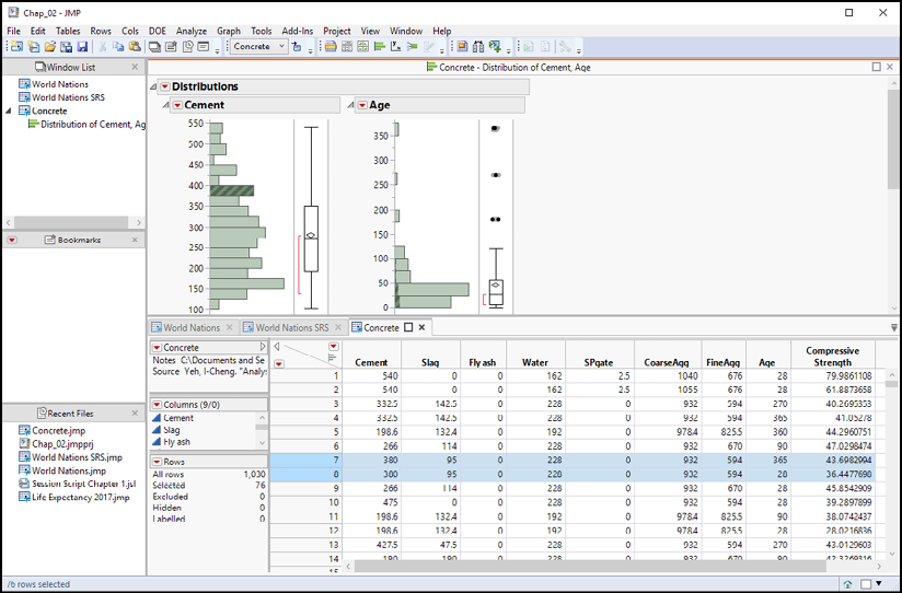
Finally, look at the data table. Within the data grid, several visible rows are highlighted. All of them share the same value of Cement. Within the Rows panel, we see that we have now altered the row state of 76 rows by selecting them.
Look more closely at rows 7 and 8, which are the first two of the selected rows. Both represent seven-part mixtures following the same recipe of the seven materials. Observation #7 was taken at 365 days and observation #8 at 28 days. These observations are not listed chronologically, but rather are a randomized sequence typical of an experimental data table.
Row 16 is the next selected row. This formulation shares several ingredients in the same proportion as rows 7 and 8, but the amounts of other ingredients differ. This is also typical of an experiment. The researcher selected and tested different formulations. Because the investigator, Professor Yeh, manipulated the factor values, we find this type of repetition within the data table. And because Professor Yeh was able to select the factor values deliberately and in a controlled way, he was able to draw conclusions about which mixtures will yield the best compressive strength.
12. Before proceeding to the next section, restore the Distribution report to its original position. Move your cursor over the title bar Concrete – Distribution of Cement, Age. Click, drag, and release near the center of the screen over the Dock Tab drop zone.
Observational Data—An Example
Of course, experimentation is not always practical, ethical, or legal. Medical and pharmaceutical researchers must follow extensive regulations, can experiment with dosages and formulations of medications, and may randomly assign patients to treatment groups, but cannot randomly expose patients to diseases. Investors do not have the ability to manipulate stock prices (if they do and get caught, they go to prison).
Now open the data table called Stock Index Weekly. This data table contains time series data for six different major international stock markets during 2008, the year in which a worldwide financial crisis occurred. A stock index is a weighted average of the prices of a sample of publicly traded companies. In this table, we find the weekly index values for the following stock market indexes, as well as the average number of shares traded per week:
● Nikkei 225 Index – Tokyo
● FTSE100 Index – London
● S&P 500 Index – New York
● Hang Seng Index – Hong Kong
● IGBM Index – Madrid
● TA100 Index – Tel Aviv
The first column is the observation date. Note that the observations are basically every seven days after the second week. The other columns simply record the index and volume values as they occurred. It was not possible to set or otherwise control any of these values.
Survey Data—An Example
Survey research is conducted in the social sciences, in public health, and in business. In a survey, researchers pose carefully constructed questions to respondents, and then the researchers or the respondents themselves record the answers. In survey data, we often find coding schemes where categorical values are assigned numeric codes or other abbreviations. Sometimes continuous variables, like income or age, are converted to ordinal columns.
As an example of a well-designed survey data table, we have a small portion of the responses provided in the 2006 administration of the National Health and Nutrition Examination Survey (NHANES). NHANES is an annual survey of people in the U.S. that looks at their diet, health, and lifestyle choices. The Centers for Disease Control (CDC) posts the raw survey data for public access.2
1. Open the NHANES 2016 data table.
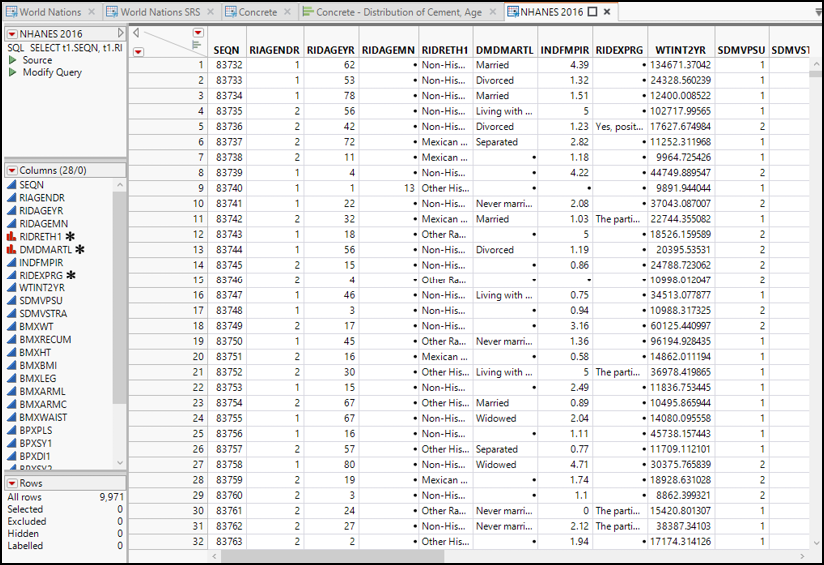
As shown in Figure 2.7, this data table contains some features that we have not seen before. As usual, each column holds observations for a single variable, but these column names are not very informative. Typical of many large-scale surveys, the NHANES website provides both the data and a data dictionary that defines each variable, including information about coding and units of measurement. For our use in this book, we have added some notations to each column.
Figure 2.7: NHANES Data Table
13. In the Columns panel, move your cursor to highlight the column named RIAGENDR and right-click. Select Column info… to open the dialog box shown in Figure 2.8.
Figure 2.8: Customizing Column Metadata
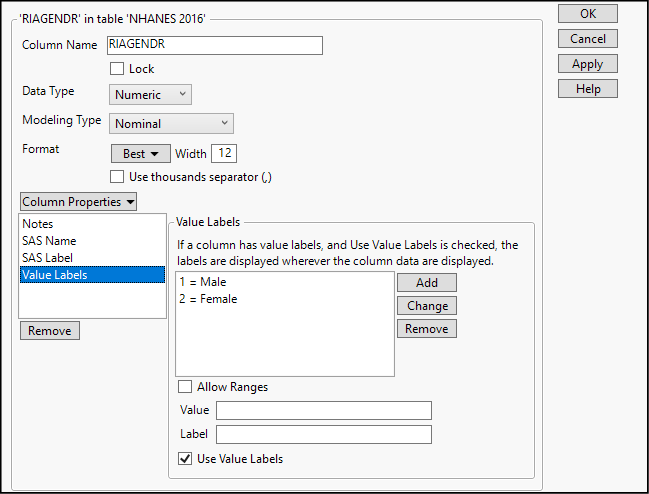
When this dialog box opens, we find that this column holds numeric data, and its modeling type is nominal—which might seem surprising since the rows in the data table all say Male or Female. In fact, the lower portion of the column info dialog box shows us what is going on here. This is an example of coded data: the actual values within the column are 1s and 2s, but when displayed in the data table, a 1 appears as the word Male and a 2 as the word Female. This recoding is a column property within JMP.
The asterisk next to RIAGENDR in the Columns panel indicates that this column has one or more special column properties defined.
14. At the bottom of the dialog box, clear the check box marked Use Value Labels and click Apply. Now, look in the Data Table (NHANES 2016 tab) and see that the column displays 1s and 2s rather than the value labels.
15. Click the word Notes under Column Properties (middle left of the dialog box). You will see a brief description of the contents of this column. As you work with data tables and create your own columns, you should get into the habit of annotating columns with informative notes.
In this table, we also encounter missing observations once again. Missing data is a common issue in survey data and it crops up whenever a respondent does not complete a question or an interviewer does not record a response. In a JMP data table, a black dot (·) indicates missing numeric data; missing character data is just a blank. As a general rule, we want to think carefully about missing observations and why they occur in a particular set of data.
For instance, look at row 1 of this data table. We have missing observations for several variables, including the columns representing respondent’s age in months (RIDAGEMN) and pregnancy status (RIDEXPRG). Further inspection shows that respondent #83732 was a 62-year-old male.
In this book, we will almost always analyze the data tables that are available at https://support.sas.com/en/books/authors/robert-carver.html. Once you start to practice data analysis on your own, you will often need to create your own data tables. Refer to Appendix B (“Data Management”) for details about entering data from a keyboard, transferring data from the web, reading in an Excel worksheet, or assembling a data table from several other data tables.
Raw Case Data and Summary Data
This book is accompanied by more than 50 data tables, most of which contain “casewise” data, meaning that each row of the data table refers to one observational unit. For example, each row of the NHANES table represents a person. Each row of the Concrete table is one batch of concrete at a moment in time. Like most statistical software, JMP is intended to analyze raw data. However, sometimes data come to us in a partially processed or summarized state. It is still possible to construct a data table and do some limited analysis of this type of data.
For example, consider public opinion surveys that have been reported in the news. Yale University and George Mason University, collaborating in the Yale Program on Climate Change Communication, published “Politics & Global Warming, April 2019.”3 The research team used “a nationally representative survey (N = 1,291 registered voters)” (Leiserowitz et al., p. 4). Among other issues, they asked respondents if they think that global warming is happening. Among all voters, 70% expressed the view that global warming is real. The researchers broke down the total sample, as shown in Table 2.1 (created from the report’s Executive Summary).
Table 2.1: Sample of U.S. Voters’ Belief that Global Warming Is Happening
|
Voter Group |
Percentage agreeing |
|
Liberal Democrats |
95 % |
|
Moderate/Conservative Democrats |
87 |
|
Liberal/Moderate Republicans |
63 |
|
Conservative Republicans |
38 |
Tables like this are common in news reports. We could easily transfer this into a data table with one major caveat that often confuses introductory students. It is crucial to understand how the layout of this table relates to its content. In JMP, we usually expect each row to represent one observational unit, each column to represent one variable, and each cell to contain one data value. This table does not satisfy these assumptions.
To see why this is not a raw data table, we should go back and think about how the raw data were generated. We know that respondents to this question—the observational units—were the 1,291 registered voters in the survey sample. The interviewers asked them many questions, and Table 2.1 tallies the responses to two of the questions. First, people reported their voting habits. The second variable is the responses those people gave when asked the question, “Do you think that global warming is happening?” Respondents could agree, disagree, or offer no opinion. Because their responses were categorical rather than numeric, this is a nominal variable.
So, how does this clarify the contents of Table 2.1? The first column lists four voter groups, ordered from most liberal to most conservative; the cell entries are unambiguously categorical. The second column is a little tricky. It appears to be continuous data, looking very much like numbers. However, these numbers are not measurements of observational units (people). They summarize some of the answers provided by the respondents, indicating the fraction of each voter group expressing agreement to the global warming question. More precisely, the values are relative frequencies of each “level” of the ordinal voter group variable. In short, this table represents one ordinal and one nominal variable, summarizing the responses of nearly 1,300 individuals who are “invisible” when the information is presented this way. In later chapters, we will learn how to use columns of frequencies. For now, our introduction to data types and sources is complete.
Now that you have completed all the activities in this chapter, use the concepts and techniques that you have learned to respond to these questions.
1. Use your primary textbook or the daily newspaper to locate a table that summarizes some data. Read the article accompanying the table and identify the variable, data type, and observational units.
2. Return to the Concrete data table. Browse through the column notes, and explain what variables these columns represent: Cement, SPgate, and FineAgg.
3. In the NHANES 2016 data table, one nominal variable appears as continuous data within the Columns panel. Find the misclassified variable and correct it by changing its modeling type to nominal.
4. The NHANES 2016 data table was assembled by scientific researchers. Why don’t we consider this data table to be experimental data?
5. Find the data table called Military. We will use this table in later chapters. This table contains rank, gender, and race information about more than a million U.S. military personnel. Use a technique presented in this chapter to create a data table containing a random sample of 500 individuals from this data table.
6. In Chapter 3, we will work with a data table called NIKKEI225. Open this table and examine the columns and metadata contained within the table. Write a short paragraph describing the contents of the table, explaining how the data were collected (experiment, observation, or survey), and define each variable and its modeling type.
7. In later chapters, we will work with a data table called Earthquakes. Open this table and examine the columns and metadata contained within the table. Write a short paragraph describing the contents of the table, explain how the data were collected (experiment, observation, or survey), and define each variable and its modeling type.
8. In later chapters, we will work with a data table called Tobacco Use. Open this table and examine the columns and metadata contained within the table. Write a short paragraph describing the contents of the table, explain how the data were collected (experiment, observation, or survey), and define each variable and its modeling type.
9. Open the Dolphins data table, which we will work with in a later chapter. What are the variable(s), observational units, and data types represented in this table?
10. Open the data table TimeUse, which we will analyze more fully in later chapters. Write a few sentences to explain the contents of the columns named marst, empstat, sleeping, and telff.
11. Open the States data table, which contains statistics about the 50 U.S. states and the District of Columbia. Write a short paragraph describing the contents of the table and, in particular, define the columns called poverty, fed_spend2010, and homicide.
Endnotes
1. In Chapter 21, we will learn how to design experiments. In this chapter, we will concentrate on the nature of experimental data.
2. Visit http://www.cdc.gov/nchs/surveys.htm to find the NHANES and other public-use survey data. Though the topic is beyond the scope of this book, readers engaged in survey research will want to learn how to conduct a database query and import the results into JMP. Interested readers should consult the section on “Importing Data” in Chapter 2 of the JMP User Guide.
3. Visit https://climatecommunication.yale.edu/publications/politics-global-warming-april-2019/ to read the full report.