
Chapter 10: Inference for a Single Categorical Variable
Statistical Inference Is Always Conditional
Using JMP to Conduct a Significance Test
Using JMP to Estimate a Population Proportion
Bootstrap Confidence Intervals (Optional; Requires JMP Pro)
Beginning with this chapter, we enter the realm of inferential statistics, where we generalize from a single sample to draw conclusions about an entire population or process. When statisticians use the term inference, it refers to two basic activities. Sometimes we want to ask whether the parameter is or is not equal to a specific value, and sometimes we want to estimate the value of a population parameter. In this chapter, we will restrict our attention to categorical dichotomous data and focus on the proportion of a population that falls in one category.
We will discuss the ideas of significance testing (often called hypothesis testing) and of confidence interval estimation. Along the way, we will illustrate these techniques and ideas using data tables with two formats common to categorical data. We often find categorical data summarized in a frequency table, but sometimes we have detailed case-by-case data.
The main message of the previous chapter is that sampling always carries the risk of inaccurately representing the larger group. We cannot eliminate the possibility that one sample will lead us to an incorrect conclusion about a population, but we can at least calibrate the risk that it will. To do so, it’s important to consider the form and origin of our data before rushing ahead to generalize from a sample. There are also other considerations to take into account and these are the topic of the next section.
Statistical Inference Is Always Conditional
Under a wide range of common conditions, good data generally leads to good conclusions. Learning to reason statistically involves knowing what those conditions are, knowing what constitutes good data, and knowing how to move logically from data to conclusions. If we are working with sample data, we need to recognize that we simply cannot infer one characteristic (parameter) of a population without making some assumptions about the nature of the sampling process and at least some of the other attributes of the population.
As we introduce the techniques of inference for a population proportion, we start with some basic conditions. If these conditions accurately describe the study and the data, the conclusions that we draw from the techniques are most likely trustworthy. If the sample departs substantially from the conditions, we should avoid generalizing from the sample to the entire population.
At a minimum, we should be able to assume the following about our sample data:
● Each observation is independent of the others. Simple random sampling assures this, and it is possible that in a non-SRS we preserve independence.
● Our sample is no more than about 10% of the population. When we sample too large a segment of the population, essentially, we no longer preserve the condition of independent observations.
We will take note of other conditions along the way, but these form a starting point. In our first example, we will look again at the pipeline safety incident data. This is not a simple random sample, even though it might be reasonable to think that one major pipeline interruption is independent of another. Because we are sampling from an ongoing nationwide process of having pipelines carry natural gas, it is also reasonable to assume that our data table is less than 10% of all disruptions that will ever occur. We will go ahead and use this data table to represent pipeline disruptions in general.
Using JMP to Conduct a Significance Test
The goal of significance testing is to make a judgment based on the evidence provided by sample data. Often the judgment implies action: is this new medication or dosage effective? Does this strategy lead to success with clients or on the field of play?
In the first chapter dealing with probability, we used data from the Pipeline and Hazardous Materials Program (PHMSA) of the U.S. Department of Transportation. The PHMSA monitors disruptions to the network of pipelines that transport natural gas. With respect to pipeline disruptions, public safety authorities might ask “Do more than 10% of disruptions involve ignition?”
The process of significance testing is bound up with the scientific method. Someone has a hunch, idea, suspicion, or concern and decides to design an empirical investigation to put the hunch to the test. As a matter of rigor and in consideration of the risk of erroneous conclusions, the test approximates the logical structure of a proof by contradiction. The investigator initially assumes the hunch to be incorrect and asks if the empirical evidence makes sense or is credible given the contrary assumption.
The hunch or idea that motivates the study becomes known as the Alternative Hypothesis usually denoted as Ha or H1. With categorical data, the alternative hypothesis is an assertion about possible values of the population proportion, p. There are two formats for an alternative hypothesis, summarized in Table 10.1.
Table 10.1: Forms of the Alternative Hypothesis
|
Name |
Example |
Usage |
|
One-sided |
Ha: p > .10 |
Investigator suspects the population proportion is more than a specific value. |
|
Ha: p < .10 |
Investigator suspects the population proportion is less than a specific value. |
|
|
Two-sided |
Ha: p ≠ .10 |
Investigator suspects the population proportion is not equal to a specific value. |
The alternative hypothesis represents the reason for the investigation, and it is tested against the null hypothesis (H0). The null hypothesis is the contrarian proposition about p asserting that the alternative hypothesis is untrue.
To summarize: we suspect, for example, that more than 10% of gas pipeline disruptions ignite. We plan to collect data about actual major pipeline incidents and count the number of fires. To test our suspicion, we initially assume that no more than 10% of the disruptions burn. Why would we begin the test in this way?
We cannot look at all incidents, but rather can observe only a sample. Samples vary, and our sample will imperfectly represent the entire population. So, we reason in this fashion:
● Assume initially that the null hypothesis is true.
● Gather our sample data and compute the sample proportion. Take note of the discrepancy between our sample proportion and the null hypothesis statement about the population.
● Knowing what we know about sampling variation, estimate the probability that a parent population like the one described in the null hypothesis would yield up a sample similar to the one that we have observed.
● Decision time:
◦ If a sample like ours would be extraordinary under the conditions described, then conclude that the null hypothesis is not credible and instead believe the alternative.
◦ If a sample like ours would not be extraordinary, then conclude that the discrepancy that we have witnessed is plausibly consistent with ordinary sampling variation.
NOTE: When we decide to reject the null hypothesis, it is fair to say that the data discredit the null assumption. However, if we decide against rejecting the null hypothesis, the sample data do not “prove” that the null hypothesis is true. The sample data simply are insufficient to conclude that the null hypothesis is false. At first, this difference might appear to be one of semantics, but it is essential to the logic of statistical inference.
In this example, suppose that our investigator wonders if the proportion of disruptions that ignite exceeds 0.10. Formally, then, we are testing these competing propositions:
|
Null hypothesis: |
H0: p ≤ .10 |
(no more than 10% of disruptions ignite) |
|
Alternative hypothesis: |
Ha: p > .10 |
(more than 10% of disruptions ignite) |
1. Open the data table Pipeline Safety.
2. Select Analyze ► Distribution to summarize the IGNITE_IND (for “ignite indicator”) column. Your results look like Figure 10.1, which was prepared in Stacked orientation to save space.
Figure 10.1: Distribution of IGNITE_IND Column
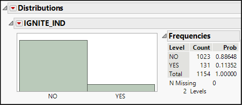
In our sample of 1,154 incidents, slightly more than 11% involved ignition. Given that disruptions had an ignition rate above 10%, should we be prepared to conclude that more than 10% of all past and future disruptions did or will ignite?
3. Click the red triangle beside IGNITE_IND and choose Test Probabilities. This opens a new panel within the report, as shown in Figure 10.2.
Figure 10.2: Specifying a Significance Test
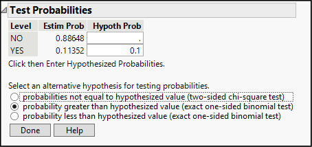
4. The upper portion of this panel displays the observed proportions of Yes and No within the sample, and leaves space for us to enter the proportions as stated in the null hypothesis. Just type .1 in the box in the second row.
5. The lower portion of the panel lists the three possible formulations of the alternative hypothesis. Click the middle option because our alternative hypothesis asserts that the population proportion is greater than 0.10, and then click Done.
There are several common ways to estimate the size of sampling error in significance tests. Most introductory texts teach a “by-hand” method based on the normal distribution because of its computational ease. Because software can do computation more easily than people can, JMP does not use the normal method, but rather selects one of two methods, depending on the alternative hypothesis. For a two-sided hypothesis, it uses a chi-square distribution, which we will study in Chapter 12. For one-sided hypotheses, it uses the discrete binomial distribution rather than the continuous normal. With categorical data, we always count the number of times an event is observed (like ignition of gas leaks). The binomial distribution is the appropriate model, and the normal distribution is a good approximation that is computationally convenient when there is no software available.
Your results should look like those in Figure 10.3. Look first to the bottom row of the results. There you will see the alternative hypothesis (p1 refers to the number that you typed in the white box above), the proportion based on the Yes values, and the p1 value that you entered. The right-most number—the P-value—is the one that is informative for the test.
Figure 10.3: Results of a Significance Test
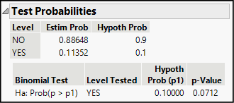
A P-value is a conditional probability. The assumed condition is that the null hypothesis is true, and the probability refers to the chance that an SRS would produce a result at least this far away from the hypothesized value. In this example, we interpret the P-value by following this logic: Our sample proportion was 0.11352, which is more than the hypothesized value of 0.10 by nearly 0.014. Assuming that the null hypothesis is true (that is, at most, 10% of all gas-line breaks ignite) and assuming we take an SRS of 1,154 incidents, the probability that we would find a discrepancy of 0.014 or more is 0.0712. This probability equates to an event that occurs 7 times out of 100.
Our decision comes down to the question, “which do we find more credible?”
● The null hypothesis is true, and our relatively high sample proportion is the result of chance.
● The reason our sample proportion is 11% is simply that the null is incorrect, and the true proportion is higher than 10%.
How shall we incorporate the P-value of 0.0712 into our decision-making? Though it has been customary to reject the null hypothesis when the P-value is smaller than 0.05, this practice has come under scrutiny.1 The reject/do not reject decision should account for (a) the consequences of mistakenly rejecting a true null hypothesis and (b) the decision maker’s tolerance for risking such an error.
The customary practice simplifies the weighing of risks and relies on a conventional standard. The standard is represented by the symbol alpha (α) and α represents our working definition of credibility. Conventionally, the default value of α is 0.05, and there is a simple decision rule. If the P-value is greater than or equal to α, we conclude that the null hypothesis is credible. If the P-value is less than α, we reject the null hypothesis as being not credible. When we reject the null hypothesis because of a very small P-value, we say that the result is statistically significant.
JMP places an asterisk (*) beside P-values that are less than 0.05 and colors them for emphasis. This convention applies to P-values in all types of significance tests. The rule is simple, but it can be hard to remember or interpret at first. The designers of JMP know this and have incorporated a reminder, as shown in this next step.
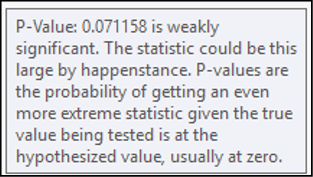
6. Move your cursor in a very small circle over the value 0.0712. Closely read the message that pops up on the screen. (See Figure 10.4.)
Figure 10.4: Pop-up Explanation of P-value
A significance test provides a yes/no response to an inferential question. For some applications, that is sufficient to the purpose. In other instances, though, the decision maker might need to estimate a proportion rather than simply determine whether it exceeds a specified limit.
We already know how to calculate the proportion of ignition incidents within our sample (about 0.11 or 11%), but that only describes the sample rather than the entire population. We shouldn’t say that 11% of all disruptions involve ignition, because that is overstating what we know. What we want to say is something like this: “Because our sample proportion was 0.81 and because we know a bit about sampling variability, we can confidently conclude that the population proportion is between ___ and ___.”
We will use a confidence interval to express an inferential estimate. A confidence interval estimates the parameter, while acknowledging the uncertainty that unavoidably comes with sampling. The technique is rooted in the sampling distributions that we studied in the prior chapter. Simply put, rather than estimating the parameter as a single value between 0 and 1, we estimate lower and upper bounds for the parameter and tag the bounded region with a specific degree of confidence. In most fields of endeavor, we customarily use confidence levels of 90%, 95%, or 99%. There is nothing sacred about these values (although you might think so after reading statistics texts); they are conventional for sensible reasons. Like most statistical software, JMP assumes we will want to use one of these confidence levels, but it also offers the ability to choose any level.
Using JMP to Estimate a Population Proportion
We already have a data table of individual incident reports. In this section, we will analyze the data in two ways. First, we will see how JMP creates a confidence interval from raw data in a data table. Next, we will see how we might conduct the same analysis if all we have is a summary of the full data table.
The Pipeline Safety data table contains raw casewise data—that is, each row is a unique observation. We will use this data table to illustrate the first method.
1. In the Distribution report, click the red triangle beside IGNITE_IND and choose Confidence Intervals ► 0.95.
A new panel will open in the results report. The confidence interval estimate for the entire population appears in the table row beginning with the word Yes, as highlighted in Figure 10.5. We find the sample proportion in the Prob(ability) column and the endpoints of the confidence interval in the Lower CI and Upper CI. Finally, the confidence level2 of 0.95 appears in the column labeled 1-Alpha. Assuming that our sample meets the conditions noted earlier, and given that 11.4% of the observed disruptions involved ignition, we can be 95% confident that the population-wide proportion of disruptions with ignition is between about 0.096 and 0.133.
Figure 10.5: A Confidence Interval for a Proportion
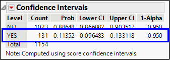
This interval estimate acknowledges our uncertainty in two respects: the width of the interval says, “this interval probably captures the actual parameter,” and the confidence level says, “there is about a 5% chance that the sample we drew unfortunately produced an interval estimate that excludes the actual parameter.”
Notice that the sample proportion of .11352 is just about midway (but not exactly) between the upper and lower CI boundaries. That is not an accident; confidence intervals are computed by adding and subtracting a small margin of error to the sample proportion. There are several common methods for estimating both the center of the interval and the margin of error. One common elementary method takes the number of observed occurrences divided by the sample size () as the center and computes the margin of error based on percentiles of the Normal distribution. JMP uses an alternative method, as noted beneath the intervals. JMP uses “score confidence intervals,” which are sometimes called the Wilson Estimator. The Wilson estimator does not center the interval at but at a slightly adjusted value.
For most practical purposes, the computational details behind the interval are less important than the assumptions required in connection with interpreting the interval. If our sample meets the two earlier conditions, we can rely on this interval estimate with 95% confidence if our sample size is large enough. Specifically, this estimation method captures the population proportion within the interval about 95% of the time if:
The sample size, n, is sufficiently large such that and .
Bootstrap Confidence Intervals (Optional; Requires JMP Pro)
What if our sample size is too small to meet this requirement? Imagine that our sample contained just 20 pipeline disruptions. With a rough estimate of 11% of incidents involving ignition, , which falls short of 5. In such a circumstance, we might well turn to a bootstrapping to estimate the sampling distribution of the proportion.
Earlier we mentioned bootstrapping in connection with the simulators to model sampling distributions. In recent years, especially in the field of machine learning, the bootstrap approach has grown in usage. We can apply the bootstrap to create a confidence interval.
To illustrate, let’s first draw a simple random sample of 20 disruptions from our data table. We will then use that sample to demonstrate the bootstrap method.
1. For reproducibility, set a random seed of 34097. We learned to do this in Chapter 8. Recall that you choose Add-Ins ► Random Seed Reset. Enter the new seed value in the dialog box.
2. Make the Pipeline_Safety data table the active tab or window.
3. Tables ► Subset. Select a random sample size of 20 and click OK.
You will now have a data table with 20 rows.
4. Analyze ► Distribution. Cast IGNITE_IND as Y.
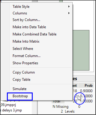
5. Move your cursor over the count or probability column in the Frequencies table in the distribution report and right-click, as shown in Figure 10.6. Select Bootstrap.
Figure 10.6: Launching the Bootstrap
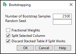
6. Bootstrapping is the process of repeatedly choosing rows from a data table with replacement. The default is to choose 2,500 samples (See Figure 10.7) of n = 20 observations. Click OK. We can then examine the distribution of the proportion of YES results to create confidence intervals.
Figure 10.7: The Bootstrapping Dialog Box
7. A new data table will open containing the relative frequencies from our first subset as well as 2,500 more bootstrap samples. Scroll through the table and notice that the proportion of YES results varies between 0.05 and 0.20. Then click the green arrow next to Distribution in the table pane of the data window.
8. Figure 10.8 shows the distribution of YES for the bootstrapped results as well as four confidence intervals.
Figure 10.8: Bootstrap Confidence Limits
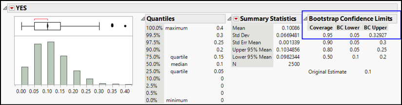
In this example, the bootstrap confidence interval is [0.05, 0.329]. By comparison to the first interval we estimated, [0.096, 0.133], the bootstrap method generates a much wider interval to cover 95% confidence. Think of the extra width as an “uncertainty premium” that we pay to work under less-than-ideal conditions. The bootstrap provides less precision, but allows us to create a useful interval from a small sample.
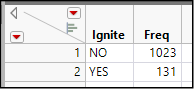
Now suppose that we did not have the complete table of data but had read a report or article that summarized this aspect of pipeline disruptions. Such a report might have stated that in the period under study, 131 pipeline disruptions ignited out of 1,154 reported incidents. So, we do not know which incidents involved fires, but we do know the total number of ignitions and the total number of incidents.
1. Create a new data table that matches Figure 10.9.
Figure 10.9: A Table for Summary Data
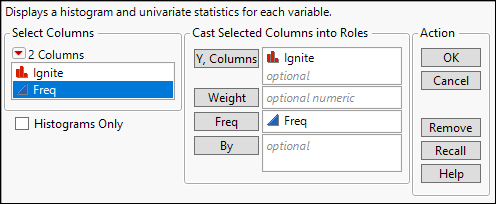
2. Select Analyze ► Distribution. As shown in Figure 10.10, cast Ignite into the Y role and identify Freq as containing the frequency counts.
Figure 10.7: Analyzing a Distribution with Summary Data
The rest of the analysis is exactly the same as described earlier. Clicking the red triangle next to Ignite opens a menu to generate the confidence interval or conduct a significance test.
Whatever we conclude, there is some chance that we have come to the wrong conclusion about the population proportion. This has nothing to do with computational mistakes or data entry errors (although it’s always wise to double check) and everything to do with sampling variability. When we construct a 95% confidence interval, we are gambling that our one sample is from among the 95% whose sample proportions lie a modest distance from the actual parameter. By bad luck, we might draw a sample from among the other 5% of possible samples.
With hypothesis tests, the situation is slightly different because we can go astray whether we reject the null hypothesis or not. If our P-value is very small, there is still a chance that we are rejecting the null hypothesis when we should not. This is called a Type I Error, and hypothesis testing is really designed to minimize the risk of encountering this situation.
Alternatively, a larger P-value (which leads us to persist in believing the null hypothesis) also carries the risk of a different (Type II) error whereby we should reject the null hypothesis, but do not because our evidence does not convince us to do so. If you can come to understand what these errors imply and why they are important to decision-making, you will more quickly come to incorporate the logic of significance testing in your own thinking.
Now that you have completed all of the activities in this chapter, use the concepts and techniques that you have learned to respond to these questions.
1. Scenario: We will continue our analysis of the pipeline disruption data.
a. Construct and interpret a 95% confidence interval for the proportion of pipeline disruptions that involved explosions (EXPLODE_IND).
b. Now construct and interpret a 90% confidence interval for the same parameter (that is, proportion of explosions).
c. In a sentence or two, explain what happens when we lower the confidence level.
d. Based on your confidence intervals, would it be credible to conclude that only 5% of all disruptions involved explosions? Explain your reasoning.
2. Scenario: You live in a community of 23,847 households. You have selected a simple random sample of 250 of these households from a printed list of addresses. Suppose that, from prior figures, you previously believed that 18% of these households have no Internet service. You suspect that more homes have recently acquired service, so that the number is now less than 18%. In your sample of 250 households, you find 35 with no service.
a. Does this situation satisfy the conditions required for statistical inference? Explain.
b. Construct a 95% confidence interval for the proportion of the community without Internet service.
c. Perform a significance test using the alternative hypothesis that is appropriate to this situation. Report on your findings, and explain your conclusion.
d. Now suppose that your sample had been four times larger, but you found the same sample proportion. In other words, you surveyed 1,000 homes and found 140 with no Internet service. Repeat parts a and b, and report on your new findings. In general, what difference does a larger sample seem to make?
3. Scenario: Recall the data in NHANES 2016. Researchers asked school-aged respondents (635 of 9,336 participants) about physical education in their schools. Recall that NHANES is a national project in the United State that randomly samples approximately 10,000 individuals, gathering comprehensive data about health, nutrition, and lifestyles. There is a new sample every two years.
a. Does the NHANES data set satisfy the conditions for inference? Explain.
b. Construct and interpret a 95% confidence interval for the population proportion of all school children who have Physical Education (PE) during the school day. (Column PAQ744). NOTE: Of the 635 school children, one did not know about PE. Use the Local Data Filter to hide and exclude that person so that we have binary responses for our sample.
c. Construct and interpret a 99% confidence interval for the same proportion using the same column. Explain fully how this interval compares to the one in part a.
d. Repeat part b using a 90% confidence level.
e. What can you say in general about the effect of the confidence level?
4. Scenario: Recall the study of traffic accidents and binge drinking introduced in Chapter 5. The data from the study were in the data table called Binge. Respondents were people ages 18 to 39 who drink alcohol.
a. Assume this is an SRS. Does this set of data otherwise satisfy our conditions for inference? Explain.
b. In that study, 213 of 3,801 respondents reported having ever been involved in a car accident after drinking. If we can assume that this is a random sample, construct and interpret a 95% confidence interval for the population proportion of all individuals who have ever been in a car accident after drinking.
c. In the same study, 485 respondents reported that they binge drink at least once a week. Based on this sample, is it credible to think that approximately 10% of the general population binge drinks at least once a week? Explain what analysis you chose to do and describe the reasoning that leads to your conclusion.
5. Scenario: Recall the study of dolphin behavior introduced in Chapter 5; this summary data is in the data table called Dolphins.
a. Assume this is an SRS. Does this set of data otherwise satisfy our conditions for inference? Explain.
b. Assuming that this is a random sample, construct and interpret a 95% confidence interval for the population proportion of dolphins who feed at a given time in the evening.
c. Based on the data in this sample, would it be reasonable to conclude that if a dolphin is observed in the morning, there is greater than a 0.5 probability that the dolphin is socializing?
6. Scenario: The data table MCD contains daily stock values for the McDonald’s Corporation for the first six months of 2019. One column in the table is called Increase, and it is a categorical variable indicating whether the closing price of the stock increased from the day before.
a. Using the data in the table, develop a 90% confidence interval for the proportion of days that McDonald’s stock price increases. Report on what you find and explain what this tells you about daily changes in McDonald’s stock.
b. Now construct a 95% confidence interval for the proportion of days that the price increases. How, specifically, does this interval compare to the one you constructed in part a?
7. Scenario: The data table TimeUse contains individual responses to a survey conducted by the American Time Use Survey in 2003, 2007, and 2017. The survey used complex sampling methods as described in Chapter 8. In all, there were 43,191 respondents, including 10,223 interviewed in 2017. For these questions, use Data Filter to restrict your analysis to the 2017 respondents. Respondents’ ages ranged from 15 to 85 years.
a. Does this data table satisfy the conditions for inference? Explain.
b. Within the chapter, all of the categorical variables that we have analyzed have been dichotomous. We can also create confidence intervals for categorical variables that have more than two levels. Construct and interpret a 95% confidence interval for the population proportion whose employment status (empstat) is “Not in labor force”.
c. Construct and interpret a 99% confidence interval for the same proportion using the same column. Explain fully how this interval compares to the one in part a. In general, what can you say about the effect of the confidence level?
d. Using the 95% confidence interval, can we conclude that less than 40% of Americans in 2017 between the ages of 15 and 85 were not in the labor force? Explain your reasoning.
8. Scenario: In this exercise, we return to the FAA Bird Strikes data table. Recall that this set of data is a record of events in which commercial aircraft collided with birds in the United States.
a. Does this data set satisfy the conditions for inference? Explain.
b. Construct and interpret a 95% confidence interval for the population proportion of flights where just one bird was struck.
c. Construct and interpret a 99% confidence interval for the same proportion using the same column. Explain fully how this interval compares to the one in part a. What can you say in general about the effect of the confidence level?
d. Based on this sample, is it credible to think that approximately 90% of reported bird strikes involve just one bird? Explain what analysis you chose to do and describe the reasoning that leads to your conclusion.
9. Scenario: The data table Hubway contains observations of 55,230 individual bike trips using the short-term rental bike-sharing system in Boston, Massachusetts. People can register with the program or simply rent a bike as needed. Within the data table, individual trips are either by Registered or Casual users.
a. Does this data table satisfy the conditions for inference? Explain.
b. Estimate (90% CI) the proportion of all Hubway trips taken by Casual users.
c. Of the 55,230 trips in the sample, 2,136 of them started at the Boston Public Library. Construct and interpret a 95% confidence interval for the proportion of all Hubway trips originating at the Library.
d. Suppose that the data table had only 5,523 rows (one-tenth the sample size) and 214 trips starting at the Library. Using this summary data, construct and interpret a 95% confidence interval for the proportion of all Hubway trips originating at the Library.
e. Compare the intervals in parts c and d. How does the size of the sample affect the confidence interval?
Endnotes
1 See Wasserstein, R.L. and Lazar, N.A. 2016, “The ASA Statement on p-Values: Context, Process, and Purpose.” The American Statistician, 70:2, 129-133, DOI: 10.1080/00031305.2016.1154108.
2 “1-Alpha” is admittedly an obscure synonym for “confidence level.” It is the complement of the significance level discussed earlier (α).