Chapter 2
Data Management
2.1 Preview
In this chapter we discuss issues relating to the management of data in GAMS models. Together with the previous chapter we complete here the introduction to GAMS, and in Section 2.4 a complete example drawn from financial planning, namely portfolio dedication, is presented.
2.2 Basics of Data Handling
It is unclear whether the heart of a financial optimization model for decision making is the data or the mathematical model. Both are indispensable for a functional and effective system: functional in that it works, and effective in that it solves the real-world problem it was designed to solve in the first place.
It is not uncommon in financial decision making for the user to deal with hundreds or even thousands of financial assets, in a variety of currencies and markets, extending over long time horizons that may run several decades into the future. Furthermore, uncertainty is prevalent and may need hundreds or thousands of scenarios to be dealt with. The user most likely will require that very large sets of data be manipulated and input to a mathematical model in order to instantiate (i.e., create a single instance of) the model that reflects the specifics of his or her problem. Hence, data handling is a critical step in all modeling applications and financial decision making is no exception.
One very important principle concerning the use of data when building models is that:
Data should be entered in its most basic form, and each data item should be entered only once.
In this way we avoid two potential pitfalls. First, entering data in its most basic form allows us to change them easily and safely, and all derived data are updated automatically. For instance, it is better to input spot rates and then use GAMS to calculate forward rates, than to input both spot and forward rates. It is better, too, to input a time series of prices and then calculate returns, than to input both prices and returns. If a price changes the GAMS code will recalculate returns, thus avoiding potential errors of data inconsistency. Second, we can isolate the input data from the algebraic representation of the model, which makes the model easier to read by other users and to be adapted to new data sets. It is good practice to keep all data separately at the beginning of a model, usually as an external input file, rather than to intersperse data with the model, and input them just before they are needed.
GAMS statements offer several formats for data as one-dimensional lists, two-dimensional tables and even multi-dimensional data structures. GAMS also offers several features to input external files so that data are kept separate from the model. Furthermore, data can be read in different formats, thus making GAMS compatible with the files generated by database management systems, spreadsheets, or other software for generating financial data. Similarly, GAMS offers features for data output and report preparation. All these features are explained next.
2.2.1 Data entry: SCALARs, PARAMETERs, and TABLEs
Numerical data in GAMS are entered as SCALAR, PARAMETER, or TABLE:
SCALAR: a single real number (no indices allowed)
PARAMETER: an indexed data collection (1 - 10 indices) of numbers
TABLE: a syntactically convenient way to declare and initialize a parameter.
All GAMS data are of double-precision, floating-point type. SCALAR, PARAMETER, and TABLE declarations differ in their initialization syntax as described in the examples below.
SCALARS

This example shows the declaration and immediate initialization of a SCALAR, tax_rate, and the declaration of another scalar, left_over, which is not immediately initialized. Initialization can occur in a later assignment statement, as shown. Scalars (or parameters) may not be used before they are initialized. The output statement (DISPLAY) is explained in Section 2.2.3.
PARAMETERS
PARAMETERS are data sets indexed by one or more indices. Indices are sets (or set aliases) that are previously declared (and initialized, if the parameter is initialized). In the following example two parameters are declared: one initialized as part of the declaration, the other left un-initialized at first, then later initialized by assignment:


An example of the declaration and initialization of a three-dimensional parameter follows:

The construct on the right means that Correlation(i,j,t) is initialized to 0.2 for bonds GOVT_1 and GOVT_2 in 2002 and to 0.3 for the 48 combinations of indices indicated.
TABLES
A TABLE declaration is just a syntactically convenient way to declare a multidimensional parameter. For instance, a two-dimensional parameter can be declared and initialized as a table:

The elements specified in a table must be positioned on the same row and column as the corresponding indices. Omitted entries correspond to zeroes. This example specifies, for instance, that and
and
All of the CashFlow entries for 2006 are 0. The elements specified must be numerical constants and cannot be expressions.
To declare parameters with three or more indices in a tabular format, use the “dot”-notation:


Tables with three or more dimensions can have set elements corresponding to any number of indices specified vertically (down along the first column) or horizontally (along the top line), separated by periods. The set elements specified must belong to the index sets, for instance, “GOVT_1”, ”GOVT_2”, “2002” correspond to sets indexed by i, j, t, respectively.
Large tables can be split using a plus sign:

In addition to specifying data directly in the source file, GAMS also interacts with databases and spreadsheets; see the GAMS User’s Guide for further information.
Exogenous versus endogenous variables
Terms such as variable or parameter mean slightly different things in different contexts. In optimization, a variable represents a decision to be made.
When GAMS solves an optimization model, the solver finds appropriate values for the variables that satisfy the model’s constraints. In economic literature such variables are sometimes called endogenous variables, in contrast to exogenous variables, or parameters. GAMS parameters may be assigned and modified as part of the model setup, and therefore act somewhat like ordinary programming language variables, but once the model is being solved they are fixed for the duration of the SOLVE statement. In summary, GAMS VARIABLES are endogenous variables; SCALARs, PARAMETERs, and TABLEs are exogenous variables.
2.2.2 External data files: INCLUDE
It is good practice to gather all the data statements of a model in a separate file. This file can be created using sophisticated data management systems, such as a relational database or a spreadsheet, and then can be included in the source file of the GAMS model. In this way not only are the data kept separately from the model, but the management of files is also eased and errors avoided.
Assuming that all data are gathered together in file ModelData.inc, then the code segment
will include the data in the source file of the GAMS model.
We use the .inc extension when the file contains GAMS data structures, i.e., it includes scalars, parameters, and tables that have been properly defined in GAMS. However, it is also possible to communicate with files created with Excel or with plain text files.
GAMS communicates with Excel via GDX (GAMS Data Exchange) files. A GDX file is a file that stores the values of one or more GAMS symbols such as sets, parameters, variables, and equations. GDX files can be used to prepare data for a GAMS model, present results of a GAMS model, store results of the same model using different parameters, etc. A GDX file does not store a model formulation or executable statements. GDX files are portable between different platforms. In order to write data from GAMS to Excel, the user writes a GDX file and then reads the Excel file from the GDX file: GAMS → GDX → Excel. This is practically seamless for the user and requires few commands as discussed in the GAMS Users’s Guide. The process for importing data from an Excel file to GAMS is similar: Excel → GDX → GAMS.
Plain text files can be imported with the CSV format; CSV stands for comma-separated values, sometimes also called comma delimited. A CSV file is a specially formatted plain text file that stores spreadsheet or basic database-style information in a very simple format, with one record on each line, and each field within that record separated by a comma. It is of course important that the individual “records” within a CSV file do not contain commas, as this may break the simple formatting when using the file in another application.
CSV files are often used as a simple way to transfer a large volume of spreadsheet or database information between programs, without worrying about special file types. For example, scenario generators could be written in C, C++, Matlab, or other simulator software. It is convenient to print the results in an ASCII file and separate the records by commas. Then, using the GAMS dollar statements ONDELIM and OFFDELIM, the data can be read in the GAMS model file.
2.2.3 Output: DISPLAY and PUT
The easiest way to output data and results is the DISPLAY statement:
Scalar and parameter data are specified without indices (i.e., VarCov, not VarCov(i,j,t)). To display variables and equations, such as X or EQN, it is necessary to specify which attribute we wish to display: X.L is the level values, X.M the marginal values, and X.UP, X.LO the bounds.
The OPTION statement provides some control over the output format. OPTION DECIMALS = 8 causes data to be displayed with 8 decimals, and OPTION X:8 does the same for data related to the symbol x.
Multidimensional data are displayed in a tabular format. The option Matrix:d:r:c causes GAMS to display using d decimals, listing the last c indices across the top, the next r indices in the left-most column, and any remaining indices in separate tables. For instance, a simple DISPLAY VarCov results in:
 whereas a DISPLAY VarCov:1:1:1 results in:
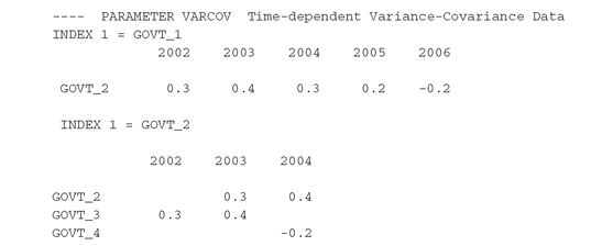 using a separate table for each value of the first index.


The PUT statement
To get complete control over output formats and to print to files (other than the listing file), the PUT statement is used. A simple example follows: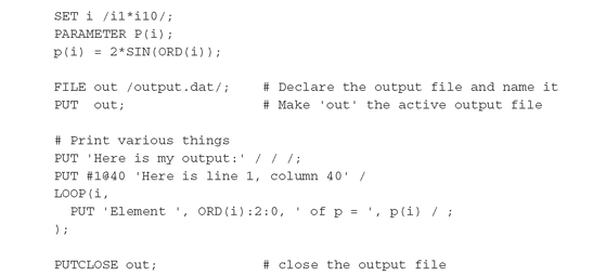

The / character in a PUT statement causes a line break; the notation #1@40 places any following output at line 1, column 40. The formatting characters in ORD(i):2:0 specify 2 positions and no decimals.
2.3 Data Generation
We have not touched upon the issue of data generation. This of course is not a problem for GAMS, and it is the user’s responsibility to generate the data that apply to the problem at hand. It is fair to assume that a user has a good understanding of the data of his or her problem before the issue of optimal decision making becomes relevant. After all, the financial optimization models aim at improving the decision making process, and whatever process was used in the past must have relied on problem data. There is a vast finance literature on pricing, forecasting, and econometric modeling, and it provides the data required for optimization studies.
The large majority of the optimization models we implement are scenario-based, and methods for scenario generation are discussed in Chapter PFO-9. Specific examples are given in the various application sections both in PFO and later in this book.
2.4 A Complete Example: Portfolio Dedication
We now describe in detail a small, but complete, GAMS model that solves the portfolio dedication Model PFO-4.2.3. The material in this section will enable the reader to understand most of the models in this book. Additional features of the language are needed to implement the more complicated case studies, but the material in the simple example presented here provides the foundation on which the more advanced models are built.
The portfolio dedication model we use is a version of the PFO model. The differences in the model implemented here compared to the model given in PFO is that the bond price Pi is included explicitly at time 0 instead of being part of the cashflow parameter F0i, and borrowing is not allowed = 0). The formal model is given as follows:


Model PFO-4.2.3 Portfolio dedication
(2.1)
(2.2)
(2.3)

(2.4)
Recall that the problem is to purchase a bond portfolio whose proceeds (coupon and principal payments) are sufficient to cover liabilities in each of a series of future time periods. Surplus cash in each period can be reinvested to the next, vt+. The optimal portfolio is the one that requires the smallest initial outlay v0 to purchase; this outlay is equal to the portfolio price (given by Σi∈U Pi xi) plus the initial reinvestment.
2.4.1 The source file
The GAMS implementation of the model DedicationNoBorrow.gms is found in Figures 2.1 and 2.2. See Section 1.3.1 for an overview of GAMS lexical conventions.
Figure 2.1: GAMS representation of the portfolio dedication model DedicationNoBorrow.gms. Data and parameter settings.
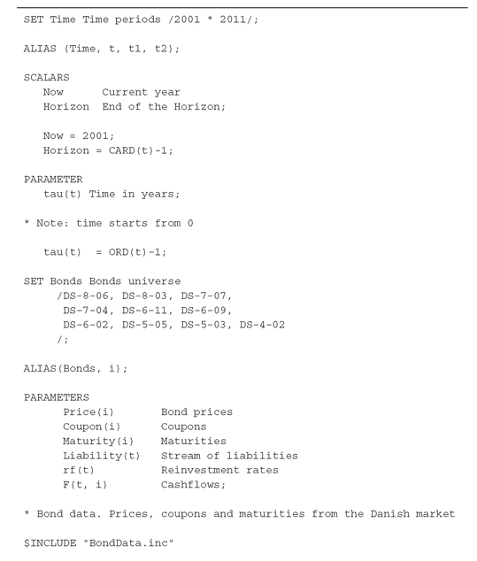
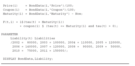
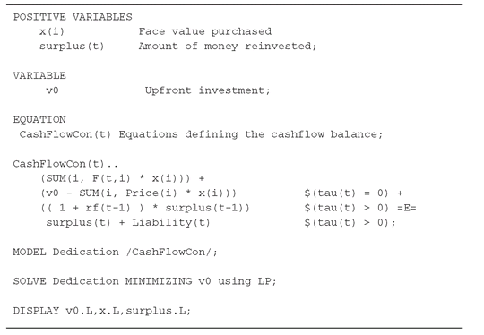
Figure 2.2: GAMS representation of the portfolio dedication model DedicationNoBorrow.gms. Variables and equations.
Sets and data
The structure of the GAMS model follows the formal model closely. First, we use Time to denote the set T = {1, 2, . . . , T }. This instance of the model covers the years 2001 through 2011, indicated by the notation /2001 * 2011/. The ALIAS statement indicates that we intend to use the index t to index the set Time. The next few lines introduce auxiliary data: the SCALAR Now that defines the starting point of the planning horizon, and a PARAMETER tau(t) that defines a mapping from the elements of the set Time into the real numbers, starting from 0. By convention, the term scalar is used for single numbers, whereas parameter usually is for vectors having one index. Multi-dimensional data can be specified as either parameters or as tables; see below.
The actual values of the parameter tau are calculated in the assignment statement tau(t) = ORD (t) - 1; the ORD function maps the index t to its ordinal value in the set Time, so that ORD(“2001”) = 1, etc. Even when set elements appear as numbers, GAMS does not by itself associate numerical values to them (except through the ORD function). Hence, the tau parameter is needed to associate the year 2001 with the numerical value 0 (time, relative to the beginning of the model’s time periods), 2002 with 1, etc.
Next, we define the bond universe U as the set Bonds and the associated index, i. The bond data are given in the TABLE BondData that follows: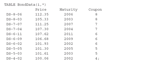

The table’s first index denotes the bonds. The asterisk as the second index indicates that this index position is not associated with any underlying set (such as Time), but can contain any identifier. In this case we need to specify each bond’s Price, Maturity year, and Coupon rate. Although we only need to know each bond’s cashflow for each year to specify the model, it is a good principle to specify only the most fundamental data in a model, and then explicitly calculate any derived data needed. Hence the calculation of the bond cashflows that follow is based on the fundamental BondData: This assignment is executed for each combination of the indices i and t. The right-hand side specifies that there is a cashflow of unity in the year where the bond matures, and a coupon payment in every year before the bond maturity, except the first. The statement illustrates the use of the conditional, or $-operator: The condition on its right is evaluated; if the result is true (non-zero), then the value of the operator is the expression on its left, otherwise it is 0. For readability we have extracted the bond data from the table into individual vectors Maturity, Coupon, etc.

Variables, equations, and the model
After specifying the Liability sequence and displaying the model data (which causes GAMS to print them to the listing file), we are ready to set up the actual optimization model. The notation POSITIVE VARIABLES x(i) specifies that we need variables xi ≥ 0 (note that “positive” really means “non-negative”), which denote the face value amount of each bond to purchase. The reinvestment variable is called surplus(t). GAMS requires that the model’s objective value be defined as a free variable, so we declare v0 as VARIABLE v0, having no bounds.
We then declare the model’s constraints in the EQUATION CashFlowCon(t) declaration, and define it (one for each value of t) as follows: This constraint states that the incoming cashflow for each year should match the liabilities. The definition of an equation is indicated by the “..” sequence, and = E = specifies that this is an equality constraint (as opposed to = G = or = L = for ≥ and ≤). Note the use of the $-operator to implement conditions: the bonds’ prices and v0 only occur in the constraint corresponding to time 0; the term (1+rf(t-1)) * surplus(t-1) only occurs in subsequent time periods. In this way, the constraint here actually implements both of the cashflow constraints of the formal model, i.e., for all values of t. Note also the use of the SUM(i, . . . ) operator to implement the summation Σi Fti xi,

Then we define the complete optimization model Dedication, consisting of the constraints CashFlowCon (and implicitly the variables referenced in those constraints), and ask to have the model solved, minimizing v0 and using an LP (Linear Programming) solver. Finally, we ask that the results be displayed: The final values (“levels”) of the variables v0 and xi , and the shadow prices (“marginals”) of xi as well as the dual variables corresponding to the cashflow constraints.
Note that, although a formal mathematical model often uses one-letter names, one can use more descriptive names in the GAMS model.
GAMS output
From the execution of source file DedicationNoBorrow.gsm we obtain listing file DedicationNoBorrow.lst. This file contains a wealth of information. First, the input source is listed. Any compilation errors will be highlighted here: The indication is an error 140 at the symbol typo; the actual error message appears after the listing:

140 Unknown symbol
When there are many error messages grouped together it’s worthwhile to focus on the first one in particular; the rest are often spurious messages.
Next, we find the output from the statement DISPLAY BondData, Liability;: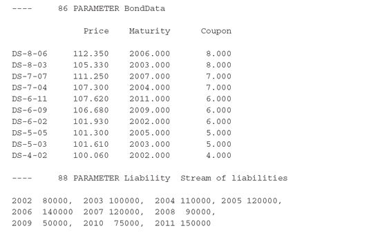

The next major sections are the equation and variable listings.
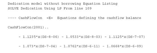
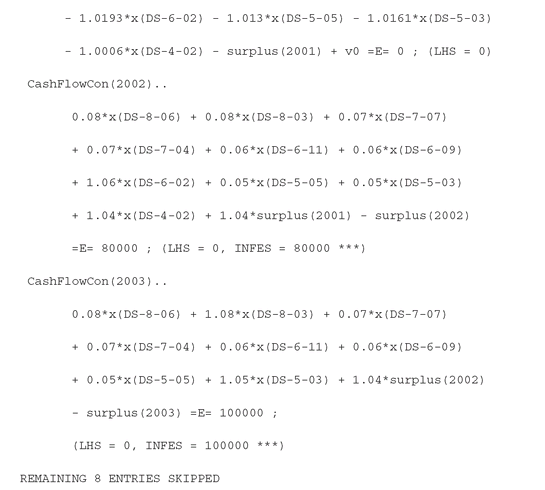
GAMS lists the equations in the model in a normalized format with variables on the left and a constant right-hand side. For each block of equations (here, CashFlowCon), only a few are listed (by default three, but this can be changed using OPTION LIMROW = n). If a variable’s coefficient is shown in parentheses the coefficient is non-constant. This only occurs in nonlinear models, and the coefficient then is the partial derivative, at the initial point, of the constraint left-hand side with respect to the variable. The listing also shows that the initial point is infeasible in these constraints (the initial point is given by the variables’ L or “level” values; see Section 1.3.5; of course, this does not mean that the model itself is infeasible!
The variable listing has the format:
 which shows that x(DS-8-06) has bounds 0 and infinity, level value 0, and that it occurs in six constraints: in CashFlowCon(2001) with coefficient -1.1235, in CashFlowCon(2002) with coefficient 0.08, etc. The number of variables in each block for which this information is shown can be specified by OPTION LIMCOL = n, and is three by default.


The model statistics show the final size of the model:

After solving the model, GAMS displays various status messages: The important things to note are that the solver terminated normally, and that the model status is “optimal.” Messages about solver problems, about infeasible or unbounded models, would also show up here. The final part of the standard output lists the model’s equations and variables (only a small part of it is shown):


The columns marked LEVEL list the values of variables or constraints left-hand sides, and the MARGINAL column lists dual information. The columns marked LOWER and UPPER list bounds on variables or constraints (the “bounds” and “level” of a constraint are explained in Section 1.3.6). A period in a numerical field means zero. Marginals may be reported as EPS; see Section 1.3.3 for details. Also, in infeasible models, equations that are not satisfied (or variables not within their bounds) are flagged INFEAS. Be aware that the cause of the infeasibility may lie elsewhere in the model.
There are various options to modify the standard output; see Table 1.6.
2.4.2 The FINLIB files
The GAMS source code and data for the models of this section are given in the following files:
• DedicationNoBorrow.gms
• BondData.inc
..................Content has been hidden....................
You can't read the all page of ebook, please click here login for view all page.
