Chapter 7
Index Funds
7.1 Preview
In this chapter we develop the GAMS models for structuring index funds. The development is based on the discussion of Chapters PFO-7 and PFO-10. The following models are discussed in this chapter and the GAMS source code for each is given in the associated FINLIB files:
Structural index funds implements a model for creating an index fund of fixed-income securities by matching two risk factors, duration and currency, based on Section PFO-7.3.1.
• StructuralModel.gms
Co-movement index funds implements a model for creating index funds by minimizing the tracking error between the portfolio return and the target index, based on Section PFO-7.3.2.
• ComovementsModel.gms
Selective hedging for index funds creates an indexation model that provides hedging for the exchange rate risk of an international portfolio, based on Section PFO-10.5.
• SelectiveHedging.gms
We implement and test the GAMS models of this chapter using two data sets stored in Excel files:
BondIndexData.xls contains 500 simulated returns of 254 bonds from three different countries, the United States, Germany, and Switzerland. It also contains scenarios of the USD/DEM and USD/CHF exchange rate, and of the return of the target index.
BroadIndexData.xls contains monthly return data for 10 asset classes over a 10-year period, including cash, stock and bond indices from the international markets. We also provide monthly data of the exchange rates covering the same period.
We use the utility GDXXRW to read the content of each file. The GAMS file Read-Data.gms in FINLIB performs the main task of reading data from the Excel files and delivering the manipulated data in GDX format. The file InputData.gdx will then be read for use by the model through the utility GDXIN.
7.2 Models for Index Funds
In this section we will customize some of the models described in Section 4.4 and Section 5.3 to deal with the specific task of building an index fund. We follow in our implementation the two approaches described in Section PFO-7.3. First, we adopt a structural approach, whereby indexed portfolios have to match some of the risk factors affecting the target index. The underlying idea is that if the portfolio and the index have the same key risk characteristics then they will have the same returns. In the co-movement approach we take next, the risk factors are not computed explicitly. Instead, we consider the index volatility as a measure of its risk factors, and the indexed portfolio is designed to be highly correlated with the target index. This is done by considering the correlations of the securities in the index and in the portfolio.
7.2.1 A structural model for index funds
A linear programming model for index funds based on the structural approach is given in Model PFO-7.3.1, and is reproduced here:


Model PFO-7.3.1 Linear program for index funds
(7.1)
(7.2)
(7.3)
(7.4)
We implement this model using bonds from the three different countries in our data set. We structure the portfolio such that the percentages of bonds in each market are equal to those reported in the reference index. Furthermore, to mirror the risk factors of the target index in more detail we segment the duration of the securities in three classes as low, medium, and high, and then constrain the portfolio to hold in each duration class the same proportion of bonds as the reference index. The model could go on to segment the available securities by, say, market segment, credit rating class, and so on, and match the proportions in each class between the target index and the portfolio. Linear programming theory tells us that the more linear constraints we add the more non-zero variables we have in the optimal solution, and this implies more diversified portfolios. However, if we have as many risk factors as the securities in the index, thus capturing residual risk as well, we end up with a portfolio that is identical to the index - which is not very useful in practice.
We declare the set BxE(BB,EE), defined over the set of bonds (BB) and currencies (EE), to carry the partition of the bonds by currencies. The set BxD(BB,DD), defined over the set of bonds (BB) and duration levels (DD), carries the partition of the bonds by duration levels.
We define by x(i) the fraction of capital to be invested in each bond. The percentage holdings are defined by CurrencyWeights(e) and DurationWeights(k).

Model PFO-7.3.3 Two-sided tracking model for index funds
(7.5)

(7.6)
(7.7)
(7.8)
The currency and duration constraints are formulated by summing the variable x(i) over the sets BxE and BxD, respectively:

The rest of the equations are similar to those described in Section 4.4.
7.2.2 A co-movement model for index funds
The co-movement approach for index funds is similar to the tracking models developed in Section 5.3.1. However, the earlier models favor upside potential, and downside risk was limited by the user’s risk appetite. In this section we are interested in replicating as close as possible the target index; hence, downside risk should be made as low as possible, which of course means that the upside potential is restricted as well. The two-sided tracking Model PFO-7.3.3 meets this requirement by limiting both upside and downside potential.
We use the same set of data as for the structural model. The two-sided tracking model is shaped through an additional constraint to limit the upside potential (see Model PFO-5.3.4 for comparison). The constraints on upside and downside are specified as follows:

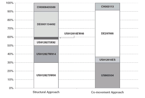
As seen in Section 5.3.1, the model is solved for decreasing values of the scalar EpsTolerance . The minimum level of EpsTolerance for which Model PFO-7.3.3 is feasible determines the indexed portfolio. The indexed portfolios obtained with the two approaches are displayed in Figure 7.1.
7.2.3 A selective hedging model for index funds
Index funds that invest in foreign country assets are exposed to exchange rate risk between the asset currency and the investor’s base currency. Currency risk can be hedged by entering in forward contracts, but this comes at a cost. In fact, a forward contract is nothing other than an insurance against unexpected changes in the value of the underlying asset.
With respect to hedging exchange rate risk, the portfolio manager can decide to fully hedge the portfolio, to leave currency risk unhedged, or to proceed with partial hedging whereby exchange rate exposure is partly covered by forward contracts. For example, a 50% hedge of the nominal amount invested in foreign countries means that only half of the total capital in foreign investments will be protected by futures. The hedging strategy whereby the hedge ratio is different for each currency included in the indexed portfolio is known as selective hedging. In selective hedging currency risk is hedged, perhaps only partially, for those currencies where data estimates dictate that currency movements are unfavorable, and remains unhedged for those currencies where the exchange rate changes appear favorable; see Chapter PFO-10 for a discussion of these issues.
Figure 7.1: Indexed portfolios obtained from the structural and the co-movement approach. The two portfolios are designed to track an index of government bonds from three major countries.
The scenario optimization model for selective hedging is displayed in Model PFO-10.5.1 (see also Section PFO-7.3).
Model PFO-10.5.1 Scenario optimization for selective hedging
(7.9)
(7.10)

(7.11)
(7.12)
The model is implemented using data from BroadIndexData.xls for the broad market indices. The risk measure we adopt in building this model is that of MAD, but similar models can be built for CVaR, or expected regret minimization, or for expected utility maximization.
The key modeling concept in implementing a selective hedging model is to split the asset allocation variable x(i) in two parts: the unhedged position variable, u(i), and the hedged position variable, h(i).
Similarly, we define by HedgedReturns(l,i) and UnhedgedReturns(l,i), respectively, the returns of the broad indices when exchange rate is hedged away through forward contracts, and the returns of the same indices when an unhedged position is taken. These are defined in GAMS as: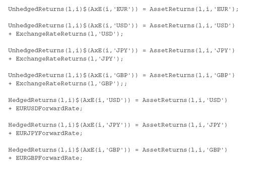

Note that, for the domestic currency EUR, the exchange rate returns are zero under all scenarios.
The equations for the selective hedging model are obtained by simply substituting in place of x(i) the two new variables u(i) and h(i). The return of the portfolio is now a function of the hedged and unhedged positions, and the MAD and return constraints become: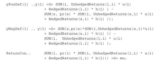

Figure 7.2: Efficient frontier of the selective hedging model vs the hedged and unhedged models. The selective hedging frontier dominates both the hedged and unhedged efficient frontiers.
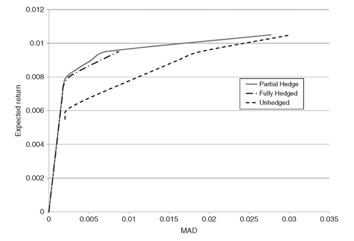
In Figure 7.2 we compare the efficient frontier obtained with the selective hedging model compared with the fully hedged and unhedged model. Note that the efficient frontier for selective hedging dominates both the fully hedged and unhedged efficient frontiers. This is as it should be, since selective hedging is the most general model, and it encompasses as special cases full hedging, no hedging and, with a small modification, partial hedging.
7.2.4 The FINLIB files
The GAMS source code and data for the models of this chapter are given in the following files:
• StructuralModel.gms
• ComovementsModel.gms
• SelectiveHedging.gms
• BondIndexData.xls
• BroadIndexData.xls
..................Content has been hidden....................
You can't read the all page of ebook, please click here login for view all page.
