Chapter 4
Portfolio Models for Fixed Income
4.1 Preview
In this chapter we develop the GAMS models for fixed-income portfolio optimization. The development is based on the discussion of Chapter PFO-4. The following models are discussed in this chapter and the GAMS source code for each is given in the associated FINLIB files:
Basics of fixed-income modeling implements simple GAMS models to perform standard financial calculations, and for bootstrapping a yield curve from bond prices.
• JDate.gms
• DiscreteFinCalc.gms
• ContinuousFinCalc.gms
• Bootstrap.gms
Dedication models are based on Section PFO-4.2. We give models for the standard portfolio dedication with borrowing and reinvestment decisions, and its extensions to maximize horizon return and to incorporate various practical considerations on the portfolio tradeability.
• Dedication.gms
• Horizon.gms
• DedicationMIP.gms
Immunization models are based on Sections PFO-4.3, PFO-4.4, and PFO-4.5. We give models for the factor immunization of portfolios of treasury bonds as well as corporate bonds. Data are given for the US, Italian, and Danish markets.
• Immunization.gms
• FactorImmunization.gms
• FactorYieldImmunization.gms
• CreditImmunization.gms
4.2 Basics of Fixed-Income Modeling
We start with some basic modeling constructs that are encountered repeatedly in the FINLIB models. In the process we develop some simple GAMS models that can be used as financial calculators.
4.2.1 Modeling time
Fixed-income models in general have long planning horizons. Even single-period models, where only today’s decision is required, rely on data extracted from a multi-year yield curve or from the prices of bonds with different maturities. The impact of today’s decision on subsequent time periods must be assessed, even if this is done in a rather simple context assuming a static yield curve and not allowing portfolio rebalancing. Hence, we need a general way to model time in GAMS.
For all our models we can assume a finite, discrete set of time points where things happen. These time instances represent the stages of the portfolio model. These may be annual, semi-annual, or even some unevenly spaced set of time points. For instance, they can be the regular intervals when coupon payments are received, or they can be the irregular intervals when a liability is due, for example, because a pension fund participant is going into retirement, an insurance claim is being filed, or a construction project installment must be paid. In all instances, they can be based upon a basic set of time points Time: The actual names of the Time elements are of no importance, and we use ALIAS(Time, t) so that t can be used as the time index. However, we need to associate the elements of the set Time with chronological time. We let tau(t) be the time, in years, relative to the starting date. It will usually be convenient to let the first time point be the starting date, and have the first element of tau equal to 0. For instance, if the element of the time set TODAY denotes the current date, then tau(TODAY) = 0. This parameter may be specified simply as above (for a model with annual stages) or explicitly by the user for a more complicated time structure:
 The Time set is intended to capture all relevant dates at which cashflows occur or when decisions can be made. Suitable subsets and data can then be defined, for instance, if only some time points are liability dates:
 These subsets can be static or dynamic (i.e., data dependent).


In many real applications, security data such as cashflows, maturity dates, and so on are given using calendar dates, represented by year, month and day of the month. Here, the GAMS calendar functions (see Table 1.4) come in handy in initializing parameters such as tau(i) above. As an example consider the following code, where the calendar dates corresponding to time points (SET Time) are given by Year, Month, and Day in TABLE TimeInfo, and then converted to years, relative to a base date: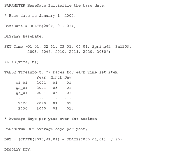
 This code is written in JDate.gms and a practical example of its use can be found in Section 4.6.


4.2.2 GAMS as a financial calculator: continuous time
With the mechanism for handling time in place, we can now specify some common formulae and expressions used in financial models. As already discussed in Chapter 2, it is good modeling practice to define as little data as possible exogenously and derive all needed data within the model. In this way, if the model parameters need to change we have to change only few instances in a data file and the rest can be computed without the need to change the model. In this case GAMS serves as a financial calculator.
The GAMS models in this chapter use exclusively continuous-time discounting. The source code for this section is found in ContinuousFinCalc.gms. Discrete-time calculations are described at the end of this section; see DiscreteFinCalc.gms.
Yields, discount factors, and forward rates
The price of a default-free, zero coupon bond that pays 1¤ at time τt is the discount factor, Dt: where rt is the spot rate; the set of spot rates for all relevant times τt is known as the spot curve. Hence, the spot rate rt is also the yield (or yield-to-maturity), yi of the default-free, zero coupon bond i. The convention is to consider yield as annualized; i.e., yi = 0.1 means a yield of 10 % per annum.
(4.1)
The GAMS code for yields and discount factors is: These formulae assume that the yield of an immediate cashflow where tau(t) = 0 is y0 = 0.

The yield-to-maturity of a bond with price P0i , which has cash payments Fti at time τt , is defined as the discount rate yi , applied to all the bond’s cash payments, that equates the bond’s present value to its price (Definition PFO-2.4.6): In general, this is a nonlinear equation in yi , and a procedure for calculating it is given in Section 4.2.3. Note that, for a zero coupon bond with face value 1¤ (i.e., Fti = 0 for all t < T , and FTi = 1), the yield-to-maturity is given in closed form as:
(4.2)

(4.3)
The forward rate from τ1 to τ2 is given by the continuous-time formulae (see Definition PFO-2.4.3 for the corresponding discrete-time formula): and is calculated in GAMS as

Present value
Consider a cashflow stream Fti which occurs at time τt . The present value of this cashflow discounted according to the term structure rt is given by: A notational difference between Definition PFO-2.4.4 and the above equation is due to the need to give numerical, chronological values to the time index as explained in the previous section. In order to correctly discount the cashflow Fti, it is important to know precisely what point in time the index t refers to. The translation from t to the chronological time τt serves this purpose. The present-value formulae are readily translated into GAMS:
 The calculations can also be based on discount factors:
 The example model ContinuousFinCalc.gms calculates the present value of a synthetic liability stream, L(t):
 We show in Section 4.2.3 how to estimate the term structure from observable bond prices.
(4.4)


Discrete-time calculations
Calculations of the yields-to-maturity, discount factors, forward rates, and present values can be calculated in discrete time as well. The discrete-time formulae are given in Section PFO-2.4.
4.2.3 Bootstrapping the term structure of interest rates
A basic problem in fixed-income analysis is that of determining a term structure from observed bond prices. That is, to determine spot rates, rt (Definition PFO-2.4.1) that are consistent with the prices Pi of a set of risk-free bonds with given coupon rates and maturities, so that:
 where Fti is the bond cashflow - principal and interest - at time t and Ti is the maturity time of bond i.

Given a set of price equations for multiple bonds i we have a nonlinear system in the rt ’s. If, for each t, we are given precisely one bond that matures at τt , then the problem can be solved in closed form. The process of recovering the spot rates from a series of prices is known as “bootstrapping.”
In general, however, we may have more than one bond with the same maturity or we may have dates when no bond matures. If there are such time points at which no bond matures or makes a cashflow payment, then the system is under-determined and we have to rely on interpolation to get corresponding rt values. The most common case of course is to have multiple observations, in which case the system is over-determined. In this case it is likely that no set of values rt exists, so that equation (4.5) is satisfied exactly for all i. A reasonable practice then is to find the spot rates that minimize the sum of the squared errors between the theoretical prices given by (4.5) and the observed market prices.
A simple model consists of minimizing the sum of the squared deviations of the present value of each bond from its price. This is formulated in GAMS by the code segment:


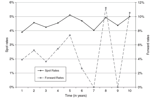
In Figure 4.1 we display spot and forward curves obtained by solving model BootstrapSimple . The spot rates show large variations at periods seven and eight, but remain positive for all the maturities. In contrast, the forward rates become negative for maturities after six years, and this is unacceptable in practice.
What we notice from this exercise is that if the number of bond observations is smaller than the number of time points on the term structure, we obtain a poor estimate of the term structure from the above procedure. In practice, it is customary to add various ad hoc constraints to ensure a reasonable result.
For example, we can impose that the forward rates are positive for each time pair (tau(t-1), tau(t)) and maturity (tau(t) > 0). We translate this into GAMS by adding the following constraints to BootstrapSimple to create a new model:


Figure 4.1: The spot rates (left axis) show a large fluctuation but remain positive for all the maturities. The one-period forward rates (right axis) are negative for some maturities.


In Figure 4.2 we display the results obtained by running model BootstrapPosForward over the same set of bond data used for model BootstrapSimple. The spot curve looks more reasonable now with rates which oscillate between 4 % to 10 %. The forward rates are positive for each maturity, however, their variation is too large to be acceptable.
To overcome this behavior, we need to smooth the forward curve such that the change between adjacent forward rates is small. For this purpose, we modify the objective function to account for the squared sum of the differences of adjacent forward rates. The term structure is obtained by properly weighting the fitting error and the curvature of the forward rates. The weight lambda trades off between the two criteria: A lambda value close to one will produce forward curves similar to that shown in Figure 4.2, while a lambda value close to zero will penalize more the fluctuations of the forward rates.

Figure 4.2: The term structure of spot rates (left axis) and of the forward rates (right axis). Although both rates are positive, their fluctuations is too large to be acceptable.

Model BootstrapSmooth is solved for different values of the weight lambda through the GAMS FOR statement: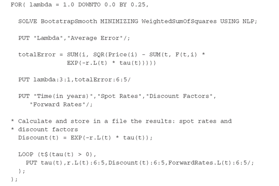

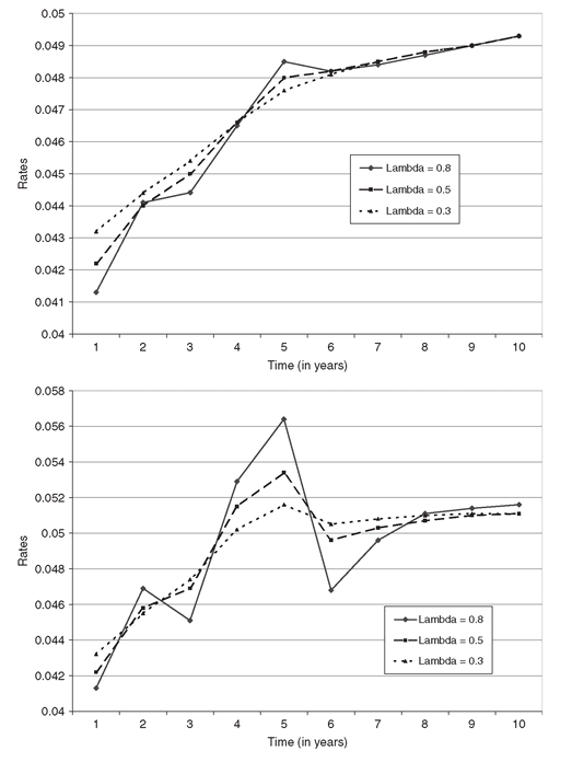
By inspecting the curves obtained from the solution with different values of lambda it is possible to select the more suitable solution. In Figure 4.3 we show the forward and spot curves for lambda equal to 0.8, 0.5, and 0.3. Note that for lambda equal to 0.8 the forward curve looks quite stable with an average fitting error equal to 0.0004.
A more general problem is to find the yield-to-maturity of a coupon bearing bond. Given the cashflows Fti of bond i, the yield-to-maturity yi satisfies the nonlinear equation:
 See Definition PFO-2.4.6 and compare to equation (4.6).

Figure 4.3: The term structure of the spot (top figure) and forward (bottom figure) rates for different values of the parameter λ. The higher the smoothing parameter 1 - λ, the more we penalize jumps between two consecutive rates, and the curves appear smoother.
The set of equations (4.6) for each i can be solved simultaneously as a square nonlinear system (i.e., having the same numbers of variables and constraints). For this purpose GAMS provides an optimizer for solving constrained nonlinear systems (CNS). Using y(i) to denote the yield-to-maturity of each bond, the following fragment of GAMS code implements the solution of the yield equations:

The structure of the file Bootstrap.gms is very simple. The data concerning the bonds used by the model are written in the file BondData.inc and they are included via the INCLUDE statement.
4.2.4 Considerations for realistic modeling
For simplicity, the models contained in this chapter ignore certain details that are crucial to realistic fixed-income applications. In particular, the models implicitly make the following assumption:
All cash inflows from the bond portfolio and outflows for liability payments occur on the same date every year.
This assumption allows the use of simple cashflow balancing constraints for each year, but it is unrealistic in practice. While it is possible to use more than one accounting date per year, one usually needs to adjust for cashflows that occur in between the accounting dates that are explicitly modeled.
On the liability side, one can easily shift liability payments to the nearest accounting date by suitably discounting by the short rate. On the asset side things are slightly more complicated. First, the purchaser of a bond has to pay, in addition to the bond’s listed price, the accrued interest, which is the part of the next coupon payment that is earned by the previous owner. For instance, if a 6 % US treasury bond with semi-annual coupon payments is purchased one month before a coupon date, the accrued interest is 5/6 of 6 %, or 5 %. This amount must be paid in addition to the bond’s listed price, but may be tax-deductible.
Second, when calculating quantities such as present values using discounting, the time until the cashflows occur needs to be adjusted accordingly. For instance, the time until the first coupon payment on the above-mentioned bond is 1/12 year, not 0 or 1 year. Ignoring this may lead to serious errors whenever one is estimating the term structure (as in Section 4.2.3), solving for cheapest portfolios (as in Section 4.3), or solving immunization models (as in Section 4.4).
4.2.5 The FINLIB files
The GAMS source code and data for the models of this section are given in the following files:
• JDate.gms
• DiscreteFinCalc.gms
• ContinuousFinCalc.gms
• Bootstrap.gms
• BondData.inc
4.3 Dedication Models
This section describes the GAMS implementations of the portfolio dedication models from Section PFO-4.2. We reproduce here Model PFO-4.2.3:
We assume that the stream of liabilities is given by and will be matched through a set of government bonds, ranging in maturity over a time period of 10 years (from 2001 to 2011). All the relevant data are from November 2001 and they are stored in BondData.inc.

Positive variables borrow(t) carry the amount of money borrowed to Liability(t). Observe that borrowing is of course not allowed in the last period - the model has no way of paying back loans after the last time period, and the optimizer would build high debt at the last time period at no cost - and this is handled using the GAMS conditional operator $ on the occurrence of the variable borrow(t) in the constraint CashFlowCon(t), describing the cashflows in each period. We also store the surplus created after the liability is paid, in the positive variable surplus(t).

There are other such conditions specified by the $-operator, to exclude parts of the constraint at the first and last time period. These kinds of boundary conditions - e.g., that borrowing is not allowed in the last time period and that there is no surplus investment before the first period - are typical of dynamic models. We use here the parameters Now to hold the numerical value of the first year of the model time period, and Horizon to hold the number of years.

After the model is solved we can use the dual prices CashFlowCon.M(t) to bootstrap the portfolio yield curve PortYield; see Section PFO-4.2.6. This is an implied yield of the optimal portfolio on the maturity dates of the liabilities.

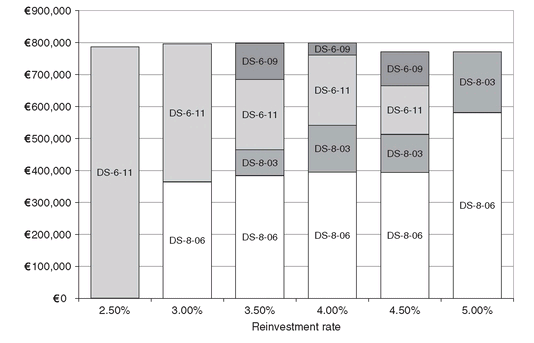
Note that the solution of Model PFO-4.2.3 depends on the level of the reinvestment rate that is a stochastic variable. In particular, the reinvestment rate is the future value of the short-term (one year in this case) rate, which is unknown today. We can have better insights by solving Model PFO-4.2.3 for different values of rf(t). In Figure 4.4 we display a set of six portfolios for constant rf(t) ranging between 2.5 % and 5 %, in incremental steps of 0.5 %.
There is a strong interplay between the reinvestment rate and the asset allocation. In particular, for reinvestment rates less than 2.5 %, the portfolio consists of only one bond (the one with the highest maturity), and since the borrowing rate is relatively cheap, liabilities are mostly covered by borrowed capital; as the reinvestment rate increases, borrowing is more and more expensive (recall that the borrowing rate is at spread over rf(t)) and buying bonds becomes more convenient. For reinvestment rates greater than 5 %, the portfolio contains no bonds and the matching of the liabilities is obtained by upfront investment reinvested at rf(t).
Figure 4.4: The composition of portfolios for different values of the reinvestment rate rf(t) shows that when borrowing is cheap the portfolio consists of the bond with the highest maturity; as rf(t) increases, the initial surplus (namely, the upfront investment), reinvested at higher rates, is sufficient to match the liabilities.
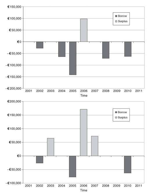
The reinvestment rate also plays a role in the schedule and amount of capital to borrow. In Figure 4.5 we show the borrowing and reinvestment amounts for each period when the reinvestment rate is equal to 3.5 % (top) and when it is equal to 4 % (bottom). For low rf(t), the proceeds from coupon payments grow at a low rate, thus more borrowing is required in each period to match the liabilities. For high rf(t), coupon payments are capitalized at higher rates and contribute more in matching the given liabilities, and in this case less borrowing is needed.
The FINLIB files
The GAMS source code and data for the models of this subsection are given in the following files:
• Dedication.gms
• BondData.inc
Figure 4.5: Borrowing and lending flow for rf(t) equal to 3.5 % (top) and 4 % (bottom).
4.3.1 Horizon return model
The model for maximizing horizon returns is a simple modification of the dedication model, see section PFO-4.2.4. We repeat Model PFO-4.2.4 here:


Model PFO-4.2.4 Portfolio horizon returns
(4.11)
(4.12)

(4.13)
(4.14)
The cash balance constraints (4.12) replace the initial cash infusion variable v0 (equation 4.8) in BondData.inc by a given Budget. The final period surplus is denoted by the variable HorizonRet, which is maximized: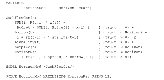

If the initial budget is larger than the optimal objective value obtained by solving the dedication model of the previous section then there will be a positive horizon return; otherwise the horizon return will simply become negative.
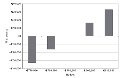
In Figure 4.6 we display the final surplus for different levels of the initial budget, and for rf(t) = 0.04. With the same rf(t), Dedication.gms finds a portfolio whose market value is equal to 798,986¤. By using as initial budget such an amount, the final horizon return is zero, as in Dedication.gms where the final return is constrained to be zero.
Figure 4.6: Surplus created by maximizing horizon returns, as a function of the initial budget.A negative (positive) final return occurs when the initial budget is smaller (larger) than the optimal objective value obtained by solving Dedication.gms.
The FINLIB files
The GAMS source code and data for the models of this subsection are given in the following files:
• Horizon.gms
• BondData.inc
4.3.2 Tradeability considerations
We now discuss the implementation of some of the tradeability considerations that occur in real-life portfolio management. In Section PFO-4.2.4 three kinds of constraints were mentioned that can be modeled using integer variables:
1. Even-lot constraints, where assets must be purchased in amounts that are “round” numbers.
2. Zero-or-range constraints, where a minimum amount, or none at all, of each asset must be purchased.
3. Fixed transaction costs, whereby a fixed cost must be paid for each asset type purchased regardless of the amount.
A model - MeanVarMip.gms - that implements zero-or-range constraints was described in Section 3.4. In this section we extend the model Dedication.gms of Section 4.3 to include even-lot purchases (with a lot-size of 1000 units), and both fixed and variable transaction costs. The complete model is found in file DedicationMIP.gms.
To address the new features of the problem we must introduce integer variables. As a consequence, the models can be considerably more time-consuming to solve than the simpler portfolio dedication or horizon return models. Even-lot purchase requirements are implemented by adding an integer variable, Y(i), for each bond i, and a constraint that the purchases x(i) must equal Y(i) times the lot-size (here in 1,000¤):

When solving integer models, one should always set upper bounds on the integer variables explicitly. It is important that these bounds be set correctly. Upper bounds that are larger than necessary may lead to excessive solution times, and bounds that are too low may exclude the optimal solution. To ensure that a feasible solution exists while restricting the bounds on Y(i) we estimate the bounds, conservatively, as: The model DedicationMIPEvenLot is made up of two sets of equations and is solved using mixed-integer programming algorithms:

The third model - DedicationMIPTrnCosts - in file DedicationMIP.gms, extends the original portfolio dedication model to include transactions costs. The formulation requires a binary variable Z(i), which takes value 1 when bond i is purchased and incurs a fixed cost of FixedCost, and is zero otherwise. The definition of this variable requires that the x(i) variables have finite upper bounds and those are set up using Y.UP(i) as above: The complete set of additional variables and constraints are:
 Finally, model DedicationMIPAll combines both models so that we have a portfolio dedication model with limits on lot size and with transaction costs.


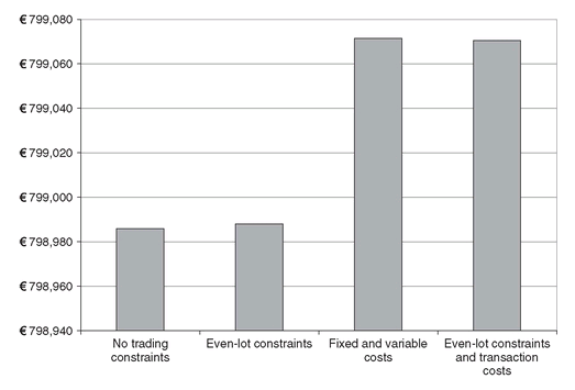
In Figure 4.7 we show the optimal portfolios for different combinations of operational constraints and transaction costs. When trading costs are included fewer bonds are included in the portfolio and the matching of the liability is done through borrowing. In this case, as well as when we add operational restrictions, the optimal solution becomes more expensive. Of course, the model will suggest borrowing money as far as this is less expensive than purchasing bonds. The difference in objective function (see Figure 4.8) is an indicator of the price we should be willing to negotiate in order to get special deals from the traders on these restrictions.
Integer programming considerations
When solving mixed-integer problems (MIP) using GAMS there are a couple of points to keep in mind. First, note that GAMS assumes an upper bound of 100 on integer variables.
Figure 4.7: Optimal portfolios for different combinations of operational constraints and transaction costs.
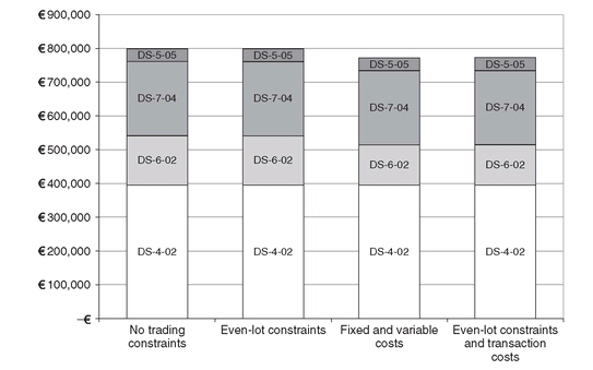
Figure 4.8: The cost of the optimal portfolio of bonds - including transaction costs - for different combinations of operational constraints and transaction costs.
This number may not be useful for some applications and it is recommended that explicit upper bounds on integer variables are specified, using the Y.UP(i) notation.
Second, we must ensure that adequate computational resources are allowed for the solvers to reach an optimal solution, and to do this we set some of the solver parameters.
The following are just illustrative; care must be exercised especially when solving large-scale integer programming models since the combinatorial nature of these problems may make them prohibitively expensive to solve: The first option OPTCR = 0 instructs the solver to settle for nothing less than the optimal integer solution, instead of the GAMS default, which is anything within 10 % of optimal. The limit on the number of iterations is set to a large value, and the CPU solution time restricted to 100 seconds.

4.3.3 The FINLIB files
The GAMS source code and data for the models of this section are given in the following files:
• Dedication.gms
• Horizon.gms
• DedicationMIP.gms
• BondData.inc
4.4 Immunization Models
In this section we implement the classic portfolio immunization (Section PFO-4.3) for managing interest rate risk.
Model PFO-4.3.1 Portfolio immunization
(4.15)
(4.16)
(4.17)
(4.18)
The GAMS model - Immunization.gms - again uses the common bonds data set contained in BondData.inc, and also uses the (derived) data calculated in Bootstrap.gms: rt , the term structure, and yi , the bond yields, contained in the parameters r(t) and YTM(t), respectively. We wrote the data in a comma-separated format (CSV) and read them using the GAMS dollar statements ONDELIM and OFFDELIM. This is a very practical way to store data when they are generated by some external software, and it is difficult to write them in the table format (for example, when the input data are made up by more than two dimensions). The GAMS statements for these two files are reported below: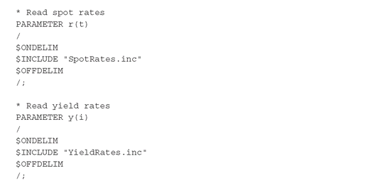 The calculations of the basic immunization determinants, i.e., the present value, Fischer-Weil duration, and convexity, are straightforward and follow directly the formulas of Section PFO-2.4.1:
 The corresponding quantities for the liability stream are calculated similarly.


Based upon these data we define two linear programming models as follows: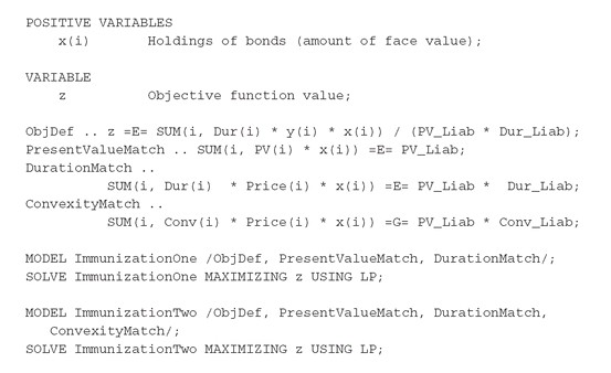 The objective here is to maximize a linear approximation of the portfolio yield; see Section 4.5.1 for an alternative.

ImmunizationOne implements present value and duration matching (Model PFO-4.3.1), and ImmunizationTwo adds a convexity matching requirement. As expected, the first model results in a barbell portfolio containing only two bonds, maturing in 2002 and 2011. This portfolio has a convexity equal to 43.237, thus making the convexity constraint of the second model inactive (the convexity of the liability is 34.005). As a consequence, both models yield the same solution.
Model PFO-4.4.1 Factor immunization
(4.19)
(4.20)
(4.21)
(4.22)
A possible alternative is to select a portfolio with the lowest possible convexity. As we know, such portfolios are less sensible to parallel shifts of the term structure when the magnitude of the shift is relatively high.

The portfolio that minimizes the convexity is made up by two bonds maturing in 2006 and 2007.
It is important to realize that no matter how large the bond universe, these three models will never return solutions containing more than two (resp. three) bonds, since they contain only two (resp. three) constraints. Despite the obvious appeal of the simple immunization models this observation points to the need for more advanced models. A significant extension that overcomes some of the limitations of immunization is given in the factor immunization model of the next section.
4.4.1 The FINLIB files
The GAMS source code and data for the models of this section are given in the following files:
• Immunization.gms
• BondData.inc
• SpotRates.inc
• YieldRates.inc
4.5 Factor Immunization Model
The factor immunization model is based on modeling and hedging against the primary factors that describe changes to the term structure, as discussed in Section PFO-4.4 and formulated in Model PFO-4.4.1.
The basic factor loadings (Definitions PFO-2.4.13 and PFO-2.4.14), βjt , describe, for each factor j, a specific change to the term structure. The reference by Dahl (1993) provides example data for the Danish term structure, and his data are used in the model below. The data consists of three factors, which together explain 99.6 % of term structure changes. The factors correspond, respectively, to the steepness, curvature, and level movements. The data are given in FactorData.inc: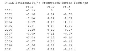

Given these data, we now calculate factor modified duration and convexity in a way similar to the basic immunization models; see Definitions PFO-4.4.1 and PFO-4.4.2. The duration and convexity data for each factor and for each bond are estimated by the following GAMS code: FactorDur(i,j) is the GAMS name for the factor modified duration of bond i with respect to factor j, and FactorConv(i,j) similarly is the factor modified convexity; similar quantities are calculated for the liability.

The factor immunization conditions are implemented through the following equations:

Two models are now defined. The first model contains only the present value and duration constraints, while the second incorporates the factor convexity constraint as well:
 Notice that the duration and convexity constraints from Immunization.gms protecting against parallel shifts are subsumed by the factors - in fact, one of the factors is almost a parallel shift. Models like these will generally result in portfolios consisting of at most κ + 1 bonds to satisfy present value and factor modified duration constraints for the κ factors, plus possibly additional bonds to satisfy the convexity constraints.


In Figure 4.9 we display the optimal portfolios for the immunization models analyzed so far. As can be seen, the simple immunization models - with and without convexity constraints - yield the same optimal portfolio. A different portfolio is obtained when the objective function minimizes the convexity of the portfolio. We are able to obtain a more diversified portfolio when we describe the term structure movements using three factors. Even with this much better diversified portfolio it may still be advisable to add limits on the very short bonds, so that duration drift is limited.
4.5.1 Direct yield maximization
The basic immunization models of Section 4.4 relied upon bond yield-to-maturity and its Fischer-Weil duration to approximate and maximize the final portfolio yield. We show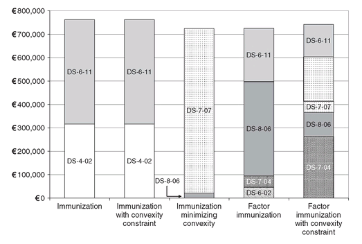 here an alternative formulation that demonstrates the power of nonlinear programming. The portfolio xi has a total yield yP which satisfies
 where Fti are the bond cashflows (coupon and principal) and Pi is the bond price. Our alternative objective is to maximize yP , called PortfolioYield in the GAMS model given in FactorYieldImmunization.gms:
Figure 4.9: Optimal portfolios for different immunization models.

(4.23)


This model has a nonlinear, non-convex objective function, and as such it is difficult to solve compared to the previous model. When solving difficult nonlinear models it is often useful to provide the solver with an approximate starting solution. This is especially true for non-convex models. In this case, we have at hand the solution of the linear approximation from the factor immunization model FactorImmunization.gms and can use it as a starting point by invoking GAMS with the “save” and “restart” options.

With this sequence of commands, the nonlinear solver starts off from the optimal solution of the linear program and it is easier to find the new optimum. In contrast, solving from scratch the model in FactorImmunization.gms may be unsuccessful.
4.5.2 The FINLIB files
The GAMS source code and data for the models of this section are given in the following files:
• FactorImmunization.gms
• FactorYieldImmunization.gms
• BondData.inc
• FactorData.inc
• SpotRates.inc
• YieldRates.inc
4.6 Factor Immunization for Corporate Bonds
This section describes a practical implementation of factor immunization models for treasury and corporate bonds. The background for the models is covered in Sections PFO-2.4.2 and PFO-4.5 and the GAMS implementations are found in the file CreditImmunization.gms.
The models correspond to Models PFO-4.5.1 and PFO-4.5.2, and they cover two credit ratings classes for corporate bonds, AAA and B3. In the first model, it is assumed that the two rating classes are uncorrelated, while the second accounts for cross-class correlation. We begin with the simpler model for uncorrelated rating classes, pointing out however that this is not a realistic assumption. Nevertheless, this model serves as a building block.
4.6.1 The model data sets
The bond universe for the model consists of 13 AAA-rated bonds and six B3-rated bonds. These are used to build portfolios immunized with respect to a liability stream using three interest-rate change factors (shift, tilt, curve). In addition, the basic data consists of yield curves (for the two ratings classes) and factor loading data. The set i accounts for the number of bonds.
The main data are given in the following GAMS data structure:
• yield(ty, class, *) contains the term (time) and interest rate for a 30-year treasury yield curve.
• LiabData(tl, *) carries year, month, day, and the amount of each liability.
• BondData(*,i,class) contains the cashflow of each bond (indexed by i for each rating class), and also their yields, price, and accrued interests. The AAA and B3 bonds are distinguished by the two rating indices.
• a(tf,class,*) stores the factor loadings for each bond.
One complication of the GAMS implementation of this model stems from the fact that the securities data (cashflows, etc.), liability data, factor loading data, and yield curve data are all given using different sets of dates. The time set for securities data is called ts, and covers 93 time points from June 1, 2000 to April 1, 2010; in stime(ts,*) we give a conversion from the time set elements to (year, month, day)-form. The time set for liability data is called tl and contains six time points over the 10-year period, none of which coincide with the dates in ts. The factor loading data are based on the set tf, and the yield curve time set is ty. The model uses interpolation to calculate the term structure for each security cashflow date, r(ts,class), and liability date, rl(ts,class). Similarly, using interpolation over time, the factor loading data are calculated from the basic factors to give sfac(ts,class,j) and lfac(tl,class,j). These in turn are used to calculate the securities and liability present values, durations, and factor durations needed for the factor immunization model.
The interpolation over time is facilitated by using the GAMS function JDATE, which takes as arguments year, month, and day-of-month, and returns the number of days since the base date. All time points are converted in years, counting from the base date, which is the first liability date. See Section 4.2.1 for an example using this procedure.
To summarize, the following quantities are calculated for use in the optimization models:
• pv(i,class) and pl(class), the present value of the assets and the liability.
• sfac(ts,class,j) and lfac(tl,class,j), the factor loadings of the bonds and the liability.
• f(i,j,class) and fl(i,class), the factor sensitivities of the bonds and the liability.
• k(i,class), the dollar duration of the bonds.
The quantities sfac(ts,class,j) and lfac(tl,class,j) correspond to the parameter βj t (see Definition PFO-2.4.14), f(i,j,class) and fl(i,class) correspond to the parameter kij (see Definition PFO-4.4.1), except that f and fl are dollar duration. The model is implemented using discrete compounding (with two annual periods) for the securities and continuous compounding for the liabilities.
Model PFO-4.5.1 Factor immunization with uncorrelated credit rating classes
(4.24)
(4.25)

(4.26)

(4.27)
4.6.2 The optimization models
The models for uncorrelated and correlated rating classes are described in Section PFO-4.5. We first implement the model where it is assumed that no correlation between the rating classes exists. In reality, the factors used are computed on the whole correlation matrix, so they do take into account the correlation between the AAA and the B3 classes. To overcome this problem, we continue to use the correlated factors, but we constrain the model to allocate the capital available in only one factor.
CreditImmunization.gms consists of several optimization models. The first one, under the name FactorCreditOne, maximizes a linear approximation to the total portfolio yield
(4.28)
Since the denominator of F(x) is constrained to be equal to the corresponding liability value (i.e., it is a constant independent of the optimal asset allocation), instead of maximizing this nonlinear fractional expression we simply minimize the numerator. The objective function is defined ignoring the minus sign using variable z, and the model is defined as follows: In addition, the model consists of the constraints, corresponding precisely to those of Model PFO-4.5.1:
 Note, however, that constraints (4.26) are not explicitly set to zero. This is because we can control the equations and the variables involved in the optimization model by simply setting the credit class exposure. As in this case, the exposure requested is only for AAA rated bonds. This approach makes the GAMS model more general. In fact, when another credit risk exposure is required, we can simply substitute its class label with the previous one. In case both exposures are required, the class label is substituted with the set name.


The second model - FactorCreditTwo - corresponds to Model PFO-4.5.2 with correlated classes. We assume that the liability is of class AAA.
Model PFO-4.5.2 Factor immunization with correlated credit rating classes
(4.29)
(4.30)

(4.31)
(4.32)
The present-value and factor-matching equations are modeled in GAMS by replacing the AAA labels with the set name class:

It is important to note that the models FactorCreditOne or FactorCreditTwo might not be feasible (as is the case for FactorCreditTwo ). In such cases, a solution that at least matches the factor immunization conditions could be suitable. Of course, the result is a portfolio with negative entries. From a financial point of view, this means that the asset must be sold short. Fund managers sometimes have the option to hold short positions. In other cases, when selling the bonds short is not possible, a short position in futures could be a practical alternative.
The model FactorCreditThree solves the system of linear equations represented by PresentValueMatchTwo and DurationMatchTwo(ja,class), where x(i,class) is not constrained to be positive. Observe that, without limiting the amount of short sales the model terminates with an unbounded solution, as the objective function can be arbitrarily minimized by shorting bonds. To this purpose, we split the decision variables x(i,class) and add a constraint to bound the amount of short sales:

If short sales are not allowed, the factor immunization model must be solved by letting DurationMatchTwo(ja,class) deviate from the levels of the liability factors.
FactorCreditFour accomplishes this task. A set of equations defines the deviation of the portfolio factors from the corresponding liability factors as follows: The objective function is modified in such a way that the sum of squared Deviations is minimized, given a penalty parameter lambda:

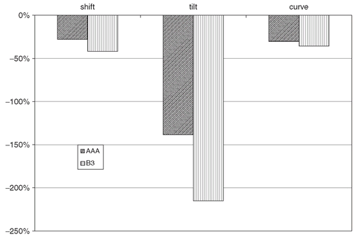
In Table 4.1 we show the asset allocation for each model discussed above. Note that the model FactorCreditOne selects only AAA since the variables activated are only those related to the AAA rating class. Model FactorCreditThree matches the factor constraints by shorting a total of 5,000¤. Finally, by allowing a mismatch between the portfolio factors and the liability factors, FactorCreditFour is able to select a portfolio with only long positions in both rating classes. This comes at a price, and in Figure 4.10 we show the factors’ mismatch in percentage of the liability target. Note how the shape risk due to the tilt factor is very poorly matched by the selected portfolio.
Table 4.1: Portfolios of bonds for the three credit factor models.
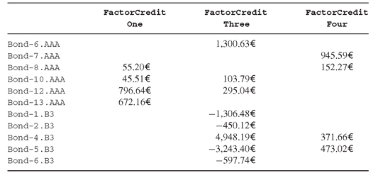
Figure 4.10: Percentage mismatch between the portfolio factors and the liability target factor values. The portfolio selected by means of FactorCreditFour is exposed to tilt risk.
4.6.3 The FINLIB files
The GAMS source code and data for the models of this section are given in the following files:
• CreditImmunization.gms
• TimeDefinitionSets.inc
• CreditYieldRates.inc
• BondAndLiabilityData.inc
• FactorLoadings.inc
..................Content has been hidden....................
You can't read the all page of ebook, please click here login for view all page.

