Chapter 8
Case Studies in Financial Optimization
8.1 Preview
In this chapter we develop the GAMS models for large-scale applications of portfolio optimization. The development is based on the discussion of Chapters PFO-10 to PFO-13. There are several important steps in going from an abstract description of the real-world problem, as described in PFO, to the implementable models we discuss here. These applications were developed by us and several collaborators over a number of years, and the models given in this chapter reflect various refinements that were developed in the implementation stage. These case studies can be used as the basis for the development of decision support systems to suit any special requirements.
The following models are discussed in this chapter and the GAMS source code for each is given in the associated FINLIB files:
International asset allocation provides models for investors that must track an international bond index while limiting their foreign exchange exposure. This model is based on Chapter PFO-10.
• BondIndex.gms
• BondIndexData.gms
Corporate bond portfolio management optimizes a portfolio of credit-risky assets following a passive, index fund, strategy. This model is based on Chapter PFO-11.
• Corporate.gms
• CorporateCVaR.gms
Minimum guarantee products develops models for the management of participating insurance policies with minimum guaranteed rate of return as discussed in Chapter PFO-12.
• GuaranteeModel.gms
Personal asset allocation provides a scenario optimization model for asset and liability management of individual investors, as described in Chapter PFO-13.
• PersonalAssetAllocation.gms
As seen in Chapter 2, GAMS can handle data having different formats. If, for example, data come from a provider and they are stored in Excel files, the GDXXRW utility is very handy for loading such data in the corresponding SETS and PARAMETERS. In general, a GDX container can also be used to store data obtained by some external programs, and then read in those data from the container itself.
However, writing directly from the simulator program to the GDX container is not always possible (we would need specific libraries to interface with). The simplest way to collect data from the simulator is to store them in plain ASCII or CSV format. In this way, GAMS can be also embedded in more complex systems where the optimization stage is only a part of the entire process.
Using GDX or ASCII files may imply a different setting of the data structures handled by GAMS. For this reason, we supply instances of the same case study when data are given in ASCII format or through a GDX container. The GDX containers are assembled starting from the plain ASCII files, so we also provide GAMS files to gather the plain data and then dump into a GDX container.
The FINLIB is also equipped with the following source files:
• GuaranteeModelData.gms
• GuaranteeModelGDX.gms
8.2 Application I: International Asset Allocation
A major Swiss bank manages several portfolios of government fixed-income securities, diversified internationally, using as a benchmark for their performance the World Government Salomon Brothers Index. Bank managers typically split the decision process into two steps: an asset allocation committee determines the exposure of the portfolio to each market, and then traders identify mispriced bonds in each market and construct the country-specific portfolio. The management is concerned with the relative lack of integration of these two functions. An optimization model could structure the decision making process, better integrate asset allocation with bond picking decisions and, perhaps, identify natural hedges among bonds in different currencies, thus resulting in improved portfolio performance.
In this section we describe the model developed to track a composite index of the international bond markets, thus providing support to the managers and traders of international portfolios. In order to cope with the volatility of the bonds and index return, we implement a mean absolute deviation MAD model over a set of scenarios of interest and exchange rates. Interest rate scenarios in multiple markets are used to estimate bond market changes in local returns, while the exchange rate scenarios convert returns to the local currency of Swiss francs. The model is based on the discussion in Section PFO-7.4 and in particular on Model PFO-7.4.4 that can incorporate operational and policy restrictions.
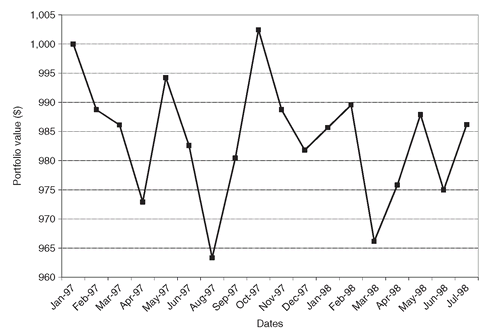
In Figure 8.1 we show the value of a 1,000 USD investment in a composite index from January 1, 1997 to July 1, 1998. This is the index we want to track. (For the purpose of this case study we do not use the Salomon Brothers global index, but a sub-index for managing a fund of investments in the US, Germany, and Switzerland.)
Scenarios of interest rates and exchange rates are generated according to the framework outlined in Section PFO-9.4.2. For each country we generate scenarios of the holding period returns of the bonds in the index and of the exchange rate against the base currency, in this case the Swiss franc (CHF). These scenarios are then combined to provide scenarios of the index. In particular, we calibrate our simulation model on a set of data obtained from the Salomon Brothers bond index for the United States, Germany, and Switzerland. The data are term structures and exchange rates from January 1990 to December 1996. Using the methodology of Section PFO-9.4.2 we estimate volatilities and correlations.
Figure 8.1: Value of a 1,000 USD investment in the composite index from January 1, 1997 to July 1, 1998.
Model PFO-7.4.4 Operational model for index funds
(8.1)
(8.2)
(8.3)

(8.4)
(8.5)
The model is run repeatedly for multiple dates. For instance, we first assume that the portfolio manager has to select a portfolio of bonds in January 1, 1997. Based on the term structure available on that date, and the historical volatilities and correlations from previous time periods, we calibrate the Monte Carlo simulation models, and generate scenarios of security and index returns. We then solve Model PFO-7.4.4 to select an indexed portfolio. The clock is then moved forward by one month and with the market data now available we can assess the performance of the portfolio. The model is run again using a new scenario set that applies to the new date. This process is repeated for each future date, using the latest information about the term structure and an updated correlation matrix.
The model is implemented in BondIndex.gms and it uses BondIndexData.gdx as its data. The GDX file is generated by BondIndexData.gms using the set of .inc files listed below. Note that some of these files contain the data generated by the simulation model. BondIndexData.gms contains the following set declarations and files: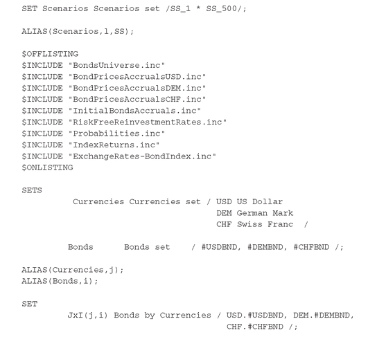

The file BondsUniverse.inc contains all the SETS that define the universe of available bonds by their CUSIP1. A sample of BondsUniverse.inc is reported here:

Note that we do not use the asset class CUSIP identifiers as labels, but use instead USD_1, USD_2, ....,USD_nn. This is because the CUSIP names given by data providers contain characters that are not allowed by GAMS (&, -, etc). Sometimes, the CUSIP is longer than 10 characters, which exceeds the GAMS limit for SET element names. With some patience it is possible to adjust these names to comply with the GAMS format. However, this is an error-prone and time-consuming procedure and the less meaningful but more mnemonic labels are used instead.
File BondPricesAccrualsXXX.inc stores bond prices (current and scenarios) and accruals, with XXX denoting the currency. The file also contains the parameter accounting for the outstanding values of each bond. Some of these bonds are callable, and under some scenarios they could be called. In these cases, the bond expires, and the outstanding value is set to zero; see the discussion on amortization factors in Section PFO-6.2.1. The cumulative risk-free interest rate, indexed by scenarios, is stored in file RiskFreeReinvestmentRates.inc, and file InitialBondsAccruals.inc stores the accrued interest for bonds held from the previous period: these data are used to determine the initial portfolio value in BondIndex.gms:

The remaining files store scenarios of index returns and exchange rates, and the probabilities associated with each scenario of interest rates and exchange rates for 500 realistic scenarios. These are sufficient to generate reasonably robust solutions, acceptable in the business setting.
8.2.1 Operational considerations
Usually, portfolio managers face a variety of operational and policy constraints. These are explicitly formulated in Model PFO-7.4.4. For example, the portfolio managers may not be allowed to trade more than 15 million CHF in Swiss bonds, since trades of this magnitude would create trading liquidity risk. Furthermore, to avoid concentration risk, the holdings in each instrument should not exceed 10 % of the total portfolio value. Once InitVal is computed, we use the UP and LO variable extensions to assign bounds on these operational requirements:

Note that, the bounds on the holdings are in percentage of the portfolio value, which is expressed in USD. Hence, to determine the amount of face value in each currency, we need to transform the USD amount using the corresponding exchange rate.
The decision variables represent the amount of face values purchased or sold, and the holdings for each instrument available in each country. It is also possible to invest in cash, which is simply one more asset returning the risk-free rate. At the end of the holding period, the portfolio is liquidated at the final prices, and the terminal value is assigned to the scenario-dependent variable FinalCash(l):
The model constraints and the objective function implementation follow along the lines of Model PFO-7.4.4:

The objective function measures the expected return of the tracking bond portfolio. Equation CashInventoryCon models the inventory of cash raised by selling bonds, the cash needed to buy bonds, and the amount of cash infused at the portfolio inception. Any remaining cash is accounted for by the variable Cash, which is invested at the risk-free rate for the next period:

The amount of face value sold and purchased has to balance out with the initial holdings and determines the holdings that will form the portfolio to be kept until the end of the horizon:
At the end of the horizon, the portfolio is liquidated (FinalCashCon(l)) and the value, under each scenario, is constrained to be as close as possible to the value of the target index, by putting a limit on the maximum deviation between the portfolio return and the index return (MADCon(l)):

The control parameter EpsTolerance determines the allowed tracking error of the portfolio return against the index return under each scenario. To determine the smallest possible value of tracking error EpsTolerance for which a feasible solution can be obtained, we set up a simple bisection algorithm that solves the model iteratively until the search interval is small enough. The extension BondIndex.MODELSTAT returns a value less or equal to 2 when a feasible solution is obtained, and it is used to guide the termination of the loop:

8.2.2 Results
The model is now validated from different perspectives. First, we carry out an ex post analysis of the performance of the portfolios built using the model during the period January 1997 to July 1998. This analysis consists of selecting a tracking portfolio starting from January 1997, on the grounds of the simulation model calibrated on January 1997. We then move the clock a month forward (February 1997), at which point we know the precise index return, security returns, and exchange rates, and can thus determine the performance of our tracking portfolio and the tracking error. This completes one step of the backtesting. We then use the term structure of February 1997 to update the volatility and correlation estimates, recalibrate the Monte Carlo simulation models, and repeat the exercise. The process is repeated until July 1998, which is the last month for which we had data when this application was first developed. It is of course straightforward to extend the GAMS data sets to update the model with more recent data.
Using the Salomon Brothers G7 index we created a composite index consisting of equal holdings in two major currencies (USD and DEM) and the currency of the sponsoring institution (CHF). In Figure 8.2, we show the growth of 1,000 USD invested in the indexed portfolios, where the holdings in any particular bond must not exceed 5%, 10%, or 20% of the total portfolio value. We observe that the models perform well in tracking the volatile index.
The Sharpe ratios are 0.199 (when imposing the 5% bounds on the holdings in any single asset), 0.208 (for 10% bounds) and 0.202 (for 20% bounds). Note that these are ex post results so we do not necessarily expect the least constrained model to reach the best Sharpe ratio. We observe instead that the tightly constrained portfolio (with bounds of 5%) lags in performance compared to the less constrained portfolios, but beyond the 10% bound there is no performance improvement. In a sense, this performance should be expected as the bounds serve to reduce concentration risk, a form of risk that is not otherwise captured in the simulation data or other model constraints. In any case, the model performance is uniformly good if we consider that the Sharpe ratio of the index is -0.068.
We impose the additional constraint that no trades should exceed 15 million CHF, due to trading liquidity requirements in the Swiss market. We also keep the bound of 10% in the holdings of any single bond, and restrict the exposure to a single currency to remain within ±15% of weight of the particular currency in the index. This set of constraints reflects essentially all operational considerations of the portfolio managers. Results are shown in Figure 8.3, and the Sharpe ratio for the operational portfolios is 0.192, with a small drop to 0.189 when the net currency exposure is limited. This figure summarizes the most encouraging statistic about the model: It shows that it is possible to build indexed portfolios that satisfy operational requirements and perform well in tracking the composite index with out-of-sample data.
We benchmark the performance of the model by evaluating its performance against random portfolios. A valuable model should produce significantly better results compared to naive approaches - such as a randomly selected portfolio. We tested the performance of randomly selected portfolios of international government bonds over the period of our backtesting. The average monthly returns and standard deviation of returns over this period are shown in Figure 8.4 for 100 randomly selected portfolios. The same information is also reported for the Salomon Brothers index and for several portfolios constructed with our models. The optimized portfolios dominate consistently in the risk-return space. It is interesting though to note that only (approximately) one quarter of the randomly selected portfolios are dominated by the index. A manager who selects bonds by throwing darts at the bond pages is likely to perform well against the broad market index but not against competitors who use sophisticated models.
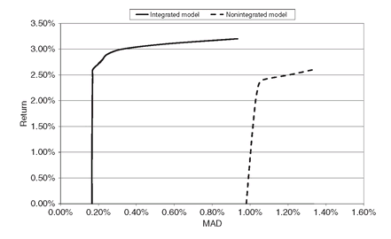
Finally, we test the efficacy of the integrated indexation model. To this end, we develop efficient frontiers using both the integrated and the nonintegrated models; see Section PFO-7.4. For the nonintegrated models, we first solve the asset allocation model and set the currency exposure to the one that yields the highest expected return. We then develop the efficient frontier of the portfolios in the three currencies such that the total exposure in each currency is equal to that determined by the asset allocation model. Figure 8.5 shows the efficient frontiers obtained with both the integrated and the nonintegrated models, and we note that the integration entails considerable benefits for the portfolio managers, by substantially reducing the volatility of the portfolio returns while also somewhat increasing the expected return.
Figure 8.2: Value of a 1,000 USD investment in the composite index, and in indexed portfolioswith bond holdings limited to 5%, 10%, and 20%, respectively, of the total portfolio value. (The figure at the bottom shows the monthly [annualized] tracking error of the portfolios with 20% limit on bond holdings.)
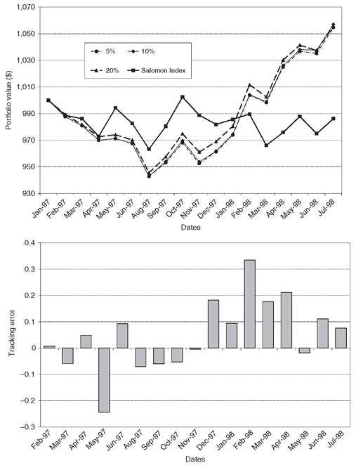
Figure 8.3: Value of a 1,000 USD investment in the composite index, and in indexed portfoliosconstrained by operational restrictions on liquidity (marked: BSI constraints) and currency exposure (marked: BSI+currency constraints). (The figure at the bottom shows the monthly [annualized] tracking error of the portfolios with liquidity and currency constraints.)
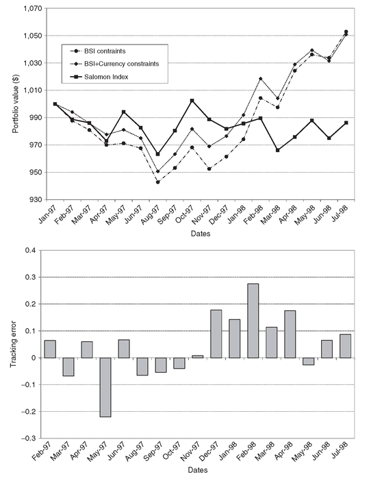
Figure 8.4: The risk-return profile of several model portfolios and 100 random portfolios during the testing period January 1997 to June 1998.
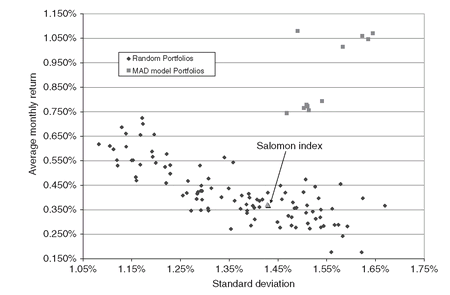
Figure 8.5: The positive effects of integrating several financial decisions in a common framework: the efficient frontier generated with the integrated model dominates the frontier generated using the nonintegrated models.
8.2.3 The FINLIB files
The GAMS source code and data for the models of this section are given in the following files:
• BondIndex.gms
• BondIndex.inc
• BondsUniverse.inc
• BondPricesAccrualsCHF.inc
• BondPricesAccrualsDEM.inc
• BondPricesAccrualsUSD.inc
• ExchangeRates-BondIndex.inc
• IndexReturns.inc
• InitialBondsAccruals.inc
• Probabilities.inc
• RiskFreeReinvestmentRates.inc
8.3 Application II: Corporate Bond Portfolio Management
Corporate bond yields are heavily affected by default and migration risk. Their return distribution is usually very skewed and fat tailed. Using data generated by the model described in Chapter PFO-11, we implement here a model to select a portfolio to track a corporate bond index (see also Chapter PFO-7). The index is built artificially by simply weighting the returns of each available bond. We take into account the hierarchial decision process performed by fund managers, and, first, we solve the strategic decision among broad asset classes, as shown below:


Model PFO-11.5.1 Strategic model for corporate indexed funds
(8.6)

(8.7)
(8.8)

(8.9)
We then use the optimal broad asset allocation, z∗, to solve the tactical asset allocation model for bond picking, Model PFO-11.5.2 as reproduced here:
Model PFO-11.5.2 Tactical model for corporate indexed funds
For eachj ∈ K, solve :


(8.10)
(8.11)
(8.12)
(8.13)
The GAMS implementation starts with the construction of the index, and the broad asset classes used for the strategic asset allocation. Of course, for real cases, these are input parameters obtained from market data.
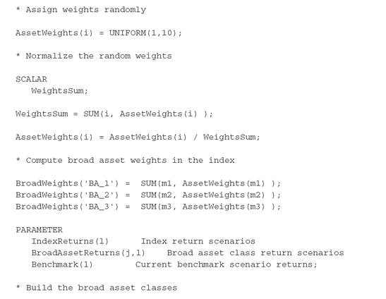

The structure of both models is very similar to that of general tracking models (see Section 5.3.1), and we briefly highlight here the main differences. In particular, we declare the definition of the portfolio return in two distinct ways to account for the strategic weights z(j), and the tactical weights x(i):

The optimal weights obtained by solving the strategic model will serve as input for the tactical model: namely, the percentage invested in each bond must add up to Current-Weight:
Models PFO-11.5.1 and PFO-11.5.2 are, respectively, implemented as follows:
To solve the StrategicModel, we have to first set the index from which the deviations are computed. In particular we have that:
For the StrategicModel, we select the optimal broad asset allocation such that deviations from the index, IndexReturns(l), are allowed within a tolerance EpsTolerance, so we have: The TacticalModel is solved for each broad asset class, by setting CurrentWeight to the optimal value obtained from StrategicModel, and setting the index to be the current asset class. For example, for the broad asset class BA_1, we have that:
 Note that we have used the same trick as in Section 3.5 to dynamically change the contents of ACTIVE. This allows us to set the domain of the securities belonging to each broad asset class.


The hierarchical decision process, and the models that follow, are shown to be sub-optimal (see Section PFO-7.4) compared to an integrated approach. The model that integrates the strategic and tactical asset allocation is given by TacticalModel, where we simply set:

Finally, as stated in Section PFO-4.2, a correct risk measure is fundamental when dealing with corporate bonds. In particular, we need a measure that penalizes appropriately extreme events, when selecting the optimal portfolio. This is accomplished using a standard Conditional VaR model, and the corresponding GAMS model is contained in Corporate-CVaR.gms. We omit its description since it follows closely the implementation given in Section 5.5.
8.3.1 The FINLIB files
The GAMS source code and data for the models of this section are given in the following files:
• Corporate.gms
• CorporateCVaR.gms
• CorporateCommonInclude.inc
• CorporateScenarios.inc
8.4 Application III: Insurance Policies with Guarantees
The model we analyze in this section is a real-world application of optimal asset allocation for insurance products with guarantee. The model is discussed in Chapter PFO-12, and includes a complete analysis of the model, together with a discussion of empirical results. Model PFO-12.4.1 is repeated here; it has linear constraints and a nonlinear objective function: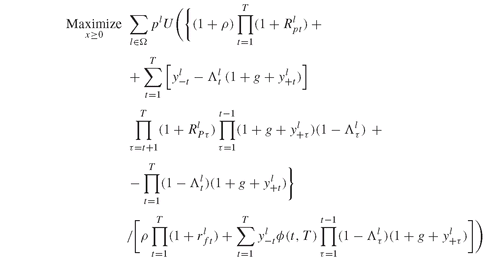


Model PFO-12.4.1 Insurance policies with guarantees
(8.14)

(8.15)
(8.16)
(8.17)
(8.18)
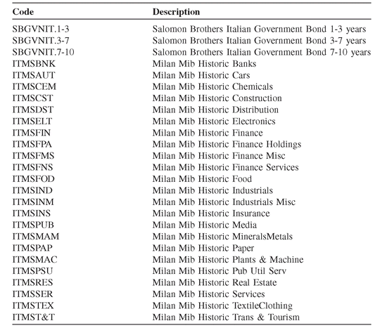
For the empirical testing of the model, the asset classes considered are the indices of the Italian stock and bond markets, as displayed in Table 8.1. We generate scenarios of asset returns by bootstrapping a set of monthly records for the 10-year period from January 1990 to February 2000. Each scenario is a sample of returns of the assets obtained by sampling historical data. For each date in our sample, we read the returns of all assets during the month prior to that date, and this is one scenario of returns. Note that, with this approach, the correlations among asset classes are preserved. See Chapter PFO-9 for a discussion of scenario generation methods, and Section PFO-9.4.1 for the bootstrapping method used to generate the scenarios in this application.
In file GuaranteeCommonInclude.inc we declare the relevant SETS and SCALARS as follows:


Table 8.1: Stock and bond indices of the Italian market.
The meaning of the three SETS is self-explanatory. With the SCALARS statement below, we input the parameters that will be used by the optimization model and in the post-processing phase:


The scenarios of asset returns, which are bootstrapped from the set of historical data, are stored in AssetReturns-Guarantee.inc. The parameter ar(l,t,i) has three indices to take into account the dependence of asset returns on the asset class set (i), the time set (t), and the scenarios set (l). The file PeriodicCapFactors.inc and CapFactors.inc store, respectively, the risk-free capitalization factor, rolled from period t to the end of the horizon T, φl (t, T ), and the risk-free capitalization factor over the entire horizon, φl (0, T ). Both parameters are scenario dependent and they are input to GAMS as a TABLE (respectively, they are pcf(l,t) and cf(l)).
Finally, the file AbandonProbabilities.inc contains the probability of abandoning the policy. The probability that a policyholder abandons the policy is Probability(death) + Probability(lapse). In the GAMS model, we set the lapse probabilities to zero and use probabilities of death from the Italian mortality tables.
The next fragment of code contains the VARIABLES declarations. Note that HO(i) corresponds to the asset holdings xi ; YP(l,t) and YM(l,t) correspond, respectively, to and
and :
:

We now turn to the equations that define the nonlinear programming model. The most complicated expression is the objective function (8.14). We assume a logarithmic utility function corresponding to growth-optimal policies:
To improve readability of the coding, we split OFe in three parts that represent, respectively, Equations PFO-12.27, PFO-12.17, and PFO-12.21: Note how the $-operator is used to control the domain of operation of the PROD operator to model the
 factor in Equation PFO-12.27. Since the PROD operator is executed over a t subset, we declare an alias set k and condition the operation PROD using k. For example, to implement the product operator
 we condition k to start from ORD(t)+1, thus ignoring all previous time indices. This is obtained by forcing the index k with the dollar condition k$(ORD(k)>ORD(t)). The product operator
 is displayed in the following code segment:
 Here the $-operator filters out all indices k greater than the current (ORD(t) - 1).

Constraints (8.15), (8.16) and (8.17) of the model are straightforward to implement and they are given in the following code segment:

When solving difficult nonlinear models it is a good practice to narrow the solution space and provide a good starting point. To assist the solver in finding a feasible solution, we set the level attribute (.L) of the variables to an initial value, and impose bounds on some of the variables.

In the post-optimization phase, we determine the cost of the guarantee and the net annualized after-tax certainty equivalent excess return on equity; see, respectively, Equations PFO-12.14 and PFO-12.47.


A complete analysis of the model, together with a discussion of empirical results, are given in Chapter PFO-12.
8.4.1 The FINLIB files
The GAMS source code and data for the models of this section are given in the following files:
• GuaranteeModel.gms
• GuaranteeCommonInclude.inc
• AssetReturns-Guarantee.inc
• CapFactors.inc
• PeriodicCapFactors.inc
• AbandonProbabilities.inc
8.5 Application IV: Personal Financial Planning
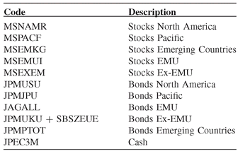
Table 8.2: Benchmarks and corresponding asset classes.
In this section we develop a scenario optimization model for asset and liability management of individual investors based on the application discussed in Chapter PFO-13, where a comprehensive analysis of the model is given together with a discussion of results obtained using a web-based system implementing the model. We consider, in particular, the optimization of the portfolio of an individual investor, who has a given level of initial wealth and wishes to reach a target goal within some time horizon. The individual must determine an asset allocation strategy so that the portfolio growth rate will be sufficient to reach the target. The model is given in PFO-Model 13.5.1 and is repeated here:
Model PFO-13.5.1 Personal financial planning
(8.19)

subject to


(8.20)

(8.21)
(8.22)
(8.23)
The set of asset classes is represented by various market benchmark indices as summarized in Table 8.2. Scenarios are generated by bootstrapping a set of historical monthly records for the 13-year period from January 1988 to February 2001. To take into account the different currencies, we considered the historical monthly records of the exchange rates for the currency of each asset class to the base currency, and proceeded to sample them in conjunction with the returns of the selected benchmarks. Each scenario is a vector of returns of the assets obtained by sampling returns that were observed during this period.
The GAMS model is run with a fixed planning horizon (nbryears), target growth rate (grr), and risk tolerance (lambda). These data are stored in PersonalCommonInclude.inc :
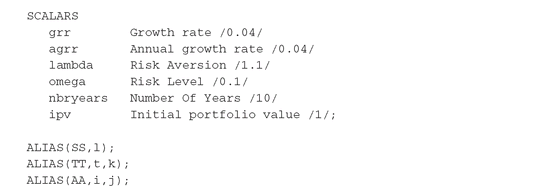


The time horizon is split in 10 time steps (t), and we test the model using 1000 scenarios (l). Given a growth rate grr and scenarios of the inflation rate, the quantity Φl(t, T) (see Definition PFO-13.28) can be computed a priori. The file LiabilityScenarios.inc contains data for the parameter lblty(l,t), accounting for the product (1 +
(1 + the file CapFactorsScenarios.inc contains data for the parameter cfs(l,t), accounting for the product
 +
+ Finally, the scenarios of price appreciation can be found in InflationScenarios.inc, and are handled through the parameter infltn(l,t).
All these files are written in comma-separated format (CSV), and the input is carried out through the INCLUDE statement, with the dollar control option ONDELIM/OFFDELIM to handle the comma delimiter:

The model for personal asset allocation uses elements of the model developed for insurance products with guarantee (see Section 8.4) and the put/call models (see Section 5.7). The variables of the problem are:

The variables YP(l,t) and YM(l,t) have the same meaning as variables and
and in Models PFO-5.7.1 and PFO-12.4.1. They are defined through the following equation:
The reward measure to be maximized is the expected value of the upside deviations from the growth rate grr; the risk measure we wish to limit is the expected value of the downside deviations from the same growth rate. Coded in GAMS they are given by: Recall that this formulation will deliver a solution with both YP(l,t) and YM(l,t) non-zero when omega is not small enough to make PUTe an active constraint; see the discussion in Section 6.2.1.

When building an efficient frontier, we can control this event through the marginal value of the PUTe equation. In fact, when the constraint is inactive, the marginal value is zero, whereas if it is active the marginal value is greater than one.
An alternative formulation of Model PFO-13.5.1 is to use an objective function that maximizes the expected upside and minimizes the expected downside, by penalizing the latter by a weight lambda strictly greater than one as follows:

We solve both models on the same set of data. Note that, either omega or lambda is set such that both YP(l,t) and YM(l,t) are non-zero (it suffices that lambda is strictly greater than one). This can be checked by displaying the parameter YpYm(l,t), which contains the products of the optimal YP.L(l,t) and YM.L(l,t).


8.5.1 The FINLIB files
The GAMS source code and data for the models of this section are given in the following files:
• PersonalAssetAllocation.gms
• PersonalCommonInclude.inc
• AssetReturns-PersonalAssetAllocation.inc
• LiabilityScenarios.inc
• InflationScenarios.inc
• CapFactorsScenarios.inc
..................Content has been hidden....................
You can't read the all page of ebook, please click here login for view all page.
