Chapter 6
Dynamic Portfolio Optimization with Stochastic Programming
6.1 Preview
In this chapter we develop the GAMS models for dynamic portfolio optimization using stochastic programming. The development is based on the discussion of Chapter PFO-6. The following models are discussed in this chapter and the GAMS source code for each is given in the associated FINLIB files:
Stochastic dedication models are based on Section PFO-6.4, and combine the static fixed-income portfolio models with scenario optimization. These models are stochastic extensions of the fixed-income models discussed in Chapter 4.
• StochDedication.gms
• StochDedicationBL.gms
Two-stage and multi-stage stochastic programs are based on Sections PFO-6.5 and PFO-6.6, and extend the scenario models analyzed in Chapter 5 to allow dynamic rebalancing of portfolios as time evolves and new information becomes known.
• TwoStageDeterministic.gms
• TwoStageStochastic.gms
• ThreeStageSPDA.gms
6.2 Dynamic Optimization for Fixed-Income Securities
As a first step towards building stochastic programming models for portfolio optimization we extend the immunization and dedication models from Sections 4.3 and 4.4 to incorporate scenarios. All the models here are built upon the finite scenario set Ω, indexed by l.
6.2.1 Stochastic dedication
We start with Model PFO-6.4.1. This is a stochastic dedication model with an objective function and risk constraints, as given in the put/call framework of Section PFO-5.7.
The model is given below:


Model PFO-6.4.1 Put/call efficient frontier for stochastic dedication
(6.1)
(6.2)
(6.3)
(6.4)

(6.5)
The model assumes that spot rates in the future are uncertain, hence, the present values of bonds as well as the liabilities are uncertain and indexed by scenario l. The model makes no assumptions on the nature of the process that generates future spot rates, and to highlight the connection to the immunization models of Sections 4.4 and 4.5, we will use the interest-rate factors given there to generate scenarios. In particular, we assume that each scenario is constructed by perturbing the short rates by some fraction of each factor. This is given in GAMS by the following code fragment: The parameter FactorWeights shows the weight of each factor in perturbing the basic spot rates, and is used to calculate the uncertain future spot rates Sr. Recall that beta (j, t) are the factor loadings (Definition PFO-2.4.14), where j denotes factors and t denotes time (see FactorData.inc). The scenario probabilities are specified by:


Here, each scenario is first given a weight, and then the probabilities are scaled to add up to one. This code segment illustrates the use of GAMS as a simulator. Of course, this scenario set may or may not make sense for a particular application. In general, scenarios are generated outside the portfolio optimization model; see Chapter PFO-9.
The next step is to calculate the present values of both sides of the balance sheet. These are scenario dependent and are computed as follows: Also recall that the price of each bond is given as the expected value over all scenarios with zero-option adjusted spread (see Definition PFO-2.4.15). In contrast with Section PFO-6.4, we use continuous discounting in our implementation, consistent with the other GAMS models implemented in this book.

The rest of the model is now quite straightforward. The key concept is to extend the scenario-dependent variables and constraints of the immunization model (Immunization.gms) from Section 4.4 by a scenario index, l: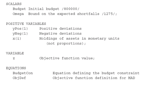


Note that for some indices l, it may happen that both yPos(l) and yNeg(l) are non-zero. This occurs because the model will find first a feasible solution, and then, if the PutCon constraint is not tight, it will increase a pair of yPos(l) and yNeg(l) variables to improve the objective.
The model in this case is exploiting the fully allowable downside risk given by Omega to top up the upside. Constraints of the form yPos(l) * yNeg(l) =E= 0 can be added to ensure that only one of the variables is non-zero, but this gives rise to a nonlinearly constrained model, which might be difficult to solve. Furthermore, since we are interested in building efficient frontiers with the smallest downside risk, we usually set ω to small values such that PutCon is active, thus avoiding the need to add nonlinear constraints. In any event, the investment decision given by x(i) will be correct, so the problem with the increase in the y variables does not pose a significant practical problem.
Alternatively, we can cast the objective function to maximize the expected upside and minimize the expected downside, by penalizing the latter by a weight lambda, strictly greater than one: The reader may wish to implement a model with such an objective function and check that both yPos(l) and yNeg(l) will be non-zero.
6.2.2 Stochastic dedication with borrowing and lending
In contrast to the stochastic dedication model, the dedication model with borrowing and lending, Model PFO-6.4.2, assumes that future cashflows and liabilities are inherently stochastic and depend on the state of the economy denoted by s for a set Σt of plausible states at period t. The uncertainty of interest rates in this case may not be the only source of uncertainty as was the assumption in stochastic dedication.
Model PFO-6.4.2 Stochastic dedication
(6.6)
(6.7)
(6.8)

(6.9)
The implementation of this model is given in StochDedicationBL.gms. We first generate random data as follows: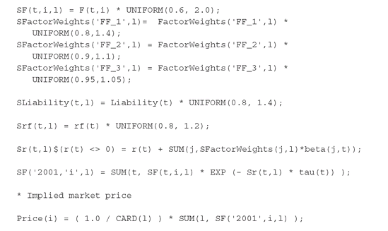

The stochastic parameters are SF (scenarios of cashflows corresponding to in the model), SLiability (scenarios of liabilities corresponding to
 , SFactorWeights (scenarios of factor weights used to generate the spot rates), Sr (scenarios of spot rates to compute the bond prices under each scenario), and Srf, the stochastic future period-by-period reinvestment yield, corresponding to
 . The implied bond prices are given by the expected value of the present values of each cashflow. Note that such quantities enter in the model as F0i, and since they represent a cost, their sign must be negated.
In realistic applications the generation of these stochastic data would require the use of suitable scenario generation methods; see Chapter PFO-9. Given scenario data, the model is now a simple extension of the dedication model of Section 4.3: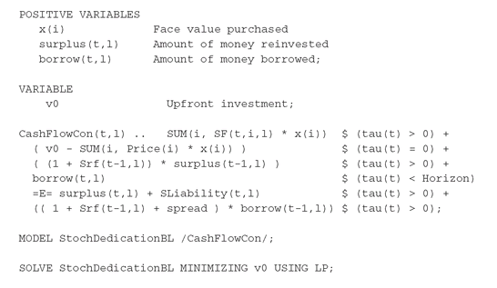

6.2.3 The FINLIB files
The GAMS source code and data for the models of this section are given in the following files:
• StochDedication.gms
• StochDedicationBL.gms
• BondData.inc
• FactorData.inc
• SpotRates.inc
6.3 Formulating Two-Stage Stochastic Programs
There are different ways to formulate stochastic models algebraically and then to implement them in GAMS. In this section, we develop a simple two-stage portfolio management problem using the so called “compact” formulation which is, as the name suggests, the most economical in terms of number of variables and constraints. Other formulations are possible, but their usefulness depends on the availability of algorithms that can exploit the algebraic structure obtained by reformulating the problem. General purpose solvers provide some options to take advantage of the model structure, but specialized solvers are needed to obtain superior performances. Just as an example, we will formulate a “split variable” model in Section 6.4, but no specific algorithms will be implemented to take advantage of the algebraic structure obtained. The interested reader can turn to PFO or to Censor and Zenios (1997) for relevant references on this issue. The general stochastic programming formulation for the portfolio optimization models implemented here is covered in Chapter PFO-6 and, in particular, Sections PFO-6.5 and PFO-6.6.
6.3.1 Deterministic and stochastic two-stage programs
We consider an investor with a budget of 10,000¤ to invest over a one-year horizon. The investment can be readjusted after six months, but no new money is injected. The objective is to maximize the expected terminal value of the final portfolio, subject to the constraint that under no circumstances must the final value be less than 11,500¤. There are three assets available for the initial (first-stage) investment: a stock, and a put and a call option on this stock. Similarly, there are three assets available for investing during the second stage: the same stock, and two new options, again a put and a call. All the options have maturities of six months.
In general we have:
• U1 and U2, the sets of assets available in stages 1 and 2.
• Vj , the final (horizon) value of asset j ∈ A2.
• P1j and P2k , the asset prices at the beginning of stages 1 and 2, for each j ∈ U1 and k ∈ U2.
• xj , first-stage holdings for each asset j ∈ U1.
• yk , second-stage holdings for each asset k ∈ U2.
At first we assume, unrealistically of course, that the future is completely known, so that we know the prices and values of all assets into the future. This results in the following deterministic dynamic problem:


(6.10)
(6.12)
(6.14)
(6.15)
Equations (6.11) and (6.12) are, respectively, the budget and the minimum return constraint. Equation (6.13) ensures that the final value of the first-stage portfolio is not less than the initial value of the second-stage portfolio, i.e., it is a rebalancing constraint.
The GAMS formulation for (6.10) - (6.15) quite straightforward: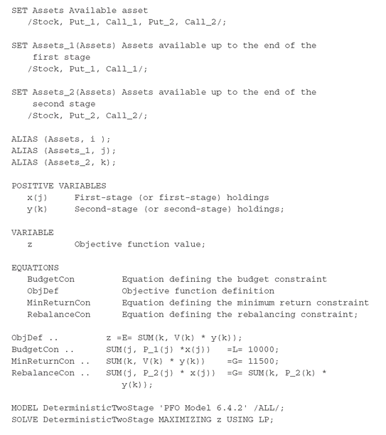

The optimal objective value of this problem is 429,414¤, which is obviously an unrealistic return from an initial budget of 10,000¤. The problem of course is that in the absence of return uncertainty, the put options in both stages are wonderful investments - too good to be true.
We introduce uncertainty into the problem using three scenarios for returns. The initial prices of the stock and the first-stage options are known, but their values at the end of the first, and at the end of the second stage, are stochastic - they differ for each of the three scenarios.
We have simply equipped all stochastic data, and the second-stage variables , with a scenario index l ∈ Ω, and also use the scenario probabilities pl , when maximizing the expected horizon value. The changes to the GAMS formulation follow those of the formal model directly. The scenario and data declarations now read:
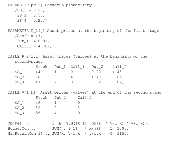


By introducing scenarios for the second stage variables, the portfolio is now more diversified. In particular, we have holdings in Stock = 198. 539 and in Put1 = 1805.933. The expected final value of the selected portfolio is 19,773.925¤.
The reader will note that equations (6.16) - (6.21) provide a general framework that can be used to extend the models developed in the previous chapter (MAD, regret minimization, expected utility maximization, etc.).
6.3.2 The FINLIB files
The GAMS source code and data for the models of this section are given in the following files:
• TwoStageDeterministic.gms
• TwoStageStochastic.gms
6.4 Single Premium Deferred Annuities: A Multi-stage Stochastic Program
We now develop a simple, yet complete, three-stage stochastic program. The resulting model is solved using various objectives, such as maximizing expected returns, maximizing the worst-case outcome, and maximizing expected utility. The GAMS code is explained along the way and the complete model is found in ThreeStageSPDA.gms.
6.4.1 Background and data
The setting for the case is an insurance company that manages retirement accounts of various types. One of their products is Single Premium Deferred Annuities, SPDA, (see Section PFO-8.3.3), where the insured (annuitant) pays a lump sum (single premium) into a managed account. The insurance company provides interest payments into this account according to certain rules (subject to caps, floors, etc.), and agrees to pay out an annual mount of money, based on the account balance, to the annuitant from age 59 onwards. The precise amounts and payment mechanisms are contractually specified. After a lock-in period (typically up to seven years) the annuitant can withdraw all or part of his account. A typical reason for terminating an account is to move the proceeds into a better paying account elsewhere.
We consider a hypothetical insurance company, which we call Winvest, that has just accepted an SPDA contract with a premium of 100,000,000¤. The risk manager of Winvest is asked to invest the premium in such a way that if interest rates increase, the company will be able to pay higher interest into the annuitants’ accounts, thus avoiding withdrawals (lapse). Recall that the value of a straight bond portfolio decreases when interest rates increase, so straight bonds are not appropriate assets for Winvest. Instead, the company is looking to derivative instruments, in particular mortgage-backed securities (MBSs) on the asset side; see Section PFO-8.3.5 for a discussion of mortgage-backed securities.
Figure 6.1: Scenario tree for a three-stage program (T = 3) having four scenarios. In this example, ξ2 has three possible realizations, and ξ3 has two possible realizations for each realization of ξ2.
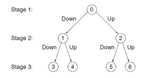
The asset and liability sides were both analyzed through interest-rate models. In our simple example model, only short rates were modeled (i.e., we use a one-factor model of the term structure with short rates as the factor) and only two stages are modeled. Today’s short rates are known, and for the particular interest-rate model employed the rates during the first stage move either up or down. In the second stage, they again move either up or down, which leads to the event tree, or scenario tree, shown in Figure 6.1, with six states and a total of four scenarios.
The changes in interest rates drive changes in the values on both the asset side (the MBSs) and the liability side (the SPDAs); see Chapter PFO-8.
The basic sets and the data in GAMS format are shown below: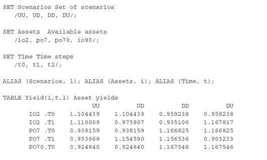
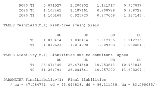


The set Scenarios defines the number of total scenarios, consisting of the up-up (denoted by UU in the GAMS model), up-down (UD), down-up (DU) and down-down (DD) sequences. The model uses a small universe of four derivatives of MBSs called IO2, PO7, PO70 and IO90, where IO is a derivative of an MBS that only contains home owners’ interest payments, and PO is a derivative of an MBS that only contains their principal payments. The model has only two stages, bounded by the three trading dates T0, T1, and T2.
The table Yield(i,t,l) contains the yields of the MBSs under each scenario, and in each stage. For instance, PO7 drops to 93.3668% of its value during the second stage under the UU scenario, i.e., from stage T1 to stage T2, but it gains 15.4590% under the UD scenario during the same stage. Apart from investing in the mortgage derivatives, one may also invest in cash. The CashYield(t,l) table shows the returns of the risk-free asset. In Liability(t,l), we store the liability payments faced by the insurance company along the way (corresponding to annuitant lapses), while FinalLiability(l) contains the outstanding liabilities originated by the future payments of the annuities to the policyholders.
We model the problem by focusing first on a single scenario. At each of the three trading dates at times T0, T1, and T2, we have the opportunity to buy, sell, or hold amounts of each of the MBSs, or of cash. We introduce the decision variables:

It is most convenient to have these variables measure value (not face value amounts) of the investments. Buying and selling securities is essentially conversion from and to cash; we therefore need to keep track of the value invested in each security and in cash, for each scenario. The following MBS balance equations keep track of the MBS holdings: The constraints (one for each stage, for each security, and for each scenario) stipulate that the amount purchased (line 1), plus the amount held from the previous stage (line 2), suitably taking into account the security’s yield during that stage, must equal the amount sold (line 3), plus the amount held into the next stage (line 4). The dollar conditions restrict the occurrence of the decision variables. For instance, one can only purchase securities prior to the last stage, and there can be holdings in securities only after the first stage.

We also need to keep track of cash, which is used for two purposes: to store value between stages, and as the intermediate numeraire when buying and selling securities. The cash balance constraints are:

Starting at line 1, the sum of incoming cash from sales of securities (less transactions costs), plus the holdings of cash from the previous stage (line 2), including interest, plus the premium of 100 mil. € received at stage T0 (line 3), must equal the total purchases (line 4), plus what is held in cash during the next stage, plus any payments of liabilities if these are included (line 5).
In the first model we use the simplest possible objective, maximizing the expected final wealth across scenarios. The latter is given as the difference between the cash accumulated and the discounted value (at stage T2) of the future payments, so we have: We introduce variables wealth(l) to collect, at the end of the horizon and under each scenario, the ratio between the cash available, cash(“t2”,l), and the final liability Final-Liability(l) . The objective value, z, to be maximized is the average over all scenarios. At this point, all the constraints and variables of the model are indexed by scenario, but there is no connection among the scenarios

Logically, we need the model to return a single, unique solution to the investment problem, regardless of the scenario that may eventually be realized. To achieve this, we add non-anticipativity constraints to the model. These are constraints that force the first-stage decisions to be identical for all scenarios. Similarly, the second-stage decisions (at stage T1) must be the same for the UU and the UD scenario - because after the first stage, the model only sees that interest rates went up, not what they will do in the second stage - and for the DU and DD scenarios. The following constraints implement these non-anticipativity requirements:

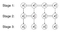
Figure 6.2: Illustration of the split-variable formulation corresponding to the scenario tree of Figure 6.1. Variables associated with each scenario/stage combination are shown. Horizontal double lines indicate non-anticipativity (equality) constraints among these variables.
This model indeed returns a solution that is implementable: At stage T0, invest 100M in PO7. If interest rates go up, then keep PO7 during the second stage; otherwise switch into IO2, which incurs a 1% loss due to transactions costs.
The formulation we have developed so far is characterized by a complete set of decision variables (buy, sell, hold) for each scenario, and additional non-anticipativity constraints that force the model not to be clairvoyant by using information that is not yet available when making first- and second-stage decisions. This formulation is known as a “split-variable” formulation - the (logically identical) first-stage variables are split up into one copy per scenario, and are then forced to be equal to each other with the additional constraints. In essence, the scenario tree of Figure 6.1 has been split up into the scenario structure shown in Figure 6.2. The decisions corresponding to each node have then been forced to agree, in accordance with the original scenario tree.
The ThreeStageSPDA.gms file contains several models that implement alternative objectives:
Model 1 implements the stochastic program with non-anticipativity constraints and no transaction costs. The portfolio is not diversified since the objective function is to maximize expected return, and hence no risk measure is considered.
Model 2 implements the same as above but with transaction costs. Again, the initial investment is not diversified, but the transaction costs reduce the rebalancing activity at stage T1.
Model 3 maximizes the worst-case outcome
Max Min Wl ,
where Wl is the scenario-dependent final wealth. The Max-Min formulation is not a linear program. We create an equivalent linear program by adding a variable WorstCase that is defined to be less than or equal to each individual outcome, and then maximize it: This model corresponds to extreme risk aversion and returns a diversified first-stage decision: 49.04% in IO2 and 50.96% in PO7.

Model 4 maximizes the expected utility, using logarithmic utility. (See Definitions PFO-2.8.6 and PFO-2.8.7.)

Here, the objective value is the expected logarithm of final wealth, and the model returns a solution with 98.1% in IO2 and 1.9% in PO7.
Model 5 is a multi-stage formulation of the tracking Model PFO-5.3.4 with limits on maximum downside risk (see Section 5.3.1). In this case we constrain the final ratios to be greater than 1.1 - a constant benchmark - by allowing a tolerance EpsTolerance so that we have:

The optimal portfolio is similar to that obtained by the worst case model (52.03% in IO2 and 47.97% in PO7). In fact, both models strongly penalize deviation from a target, which, in the worst-case model, is endogenous.
In Figure 6.3 we summarize the optimal portfolios obtained by the four models. In Figures 6.4 and 6.5 we display the optimal dynamics of the sell and buy variables. Note that purchases occur only at stage T0, and thanks to the non-anticipativity constraints, the amount purchased is the same under all scenarios. Sales occurs at stage T1, to rebalance the portfolio, and at stage T2, to liquidate the portfolio and repay liabilities. For the selling variables, the non-anticipativity constraints are active at stage T1, and the optimal decisions are pairwise equal.
6.4.2 The FINLIB files
The GAMS source code and data for the models of this section are given in the following files:
• ThreeStageSPDA.gms
Figure 6.3: The optimal holdings for the three-stage SPDA model. The models with expected wealth as objective function do not diversify the investment. By introducing a risk measure, the investment is split between two assets.
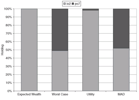
Figure 6.4: Sales under all scenarios and for each stage. Sales occur only at T1 and T2. Note that, the non-anticipativity constraints are active only at T1, and the optimal selling decisions are pairwise equal.

Figure 6.5: Purchases under all scenarios and for each stage. The non-anticipativity constraintsequalize the optimal decision under each scenario. At T1 and T2, the purchases are zero.

..................Content has been hidden....................
You can't read the all page of ebook, please click here login for view all page.
