Chapter 1
An Introduction to the GAMS Modeling System
1.1 Preview
In this chapter we introduce the high-level algebraic modeling language that will be used in the rest of this book to build financial optimization models. The basic elements of the language are given first, together with details on getting started with the language, and the FINLIB library of models are also discussed here.
1.2 Basics of Modeling
Optimization is concerned with the representation and solution of models. Models can be represented in a number of ways, and they can be solved using a number of methods or algorithms. The General Algebraic Modeling System, GAMS, is a system for formulating and solving optimization models. It consists of a language that allows a high-level, algebraic representation of mathematical models, and provides a set of solvers, i.e., numerical algorithms, to solve them.
Why use algebraic modeling? Small models are easy to formulate and solve. They have a simple structure and one can simply edit a file containing the model’s coefficients, and then call a standard linear programming solver to solve it. In fact, in the early days of optimization, models were solved using specialized matrix generators that provided the necessary input files for solvers. However, as models grow larger and become more complex, they become difficult to manage and to verify using this approach. GAMS was developed in response to the need for powerful and flexible front-end tools to manage large, real-life models. Large collections of data and models are only manageable when they possess structure, and algebra provides this structure in a well-known mathematical notation.
Conceptually, a model consists of two parts: The algebraic structure and the associated data instance. The formal linear programming model has the associated data A, b, c; see Appendix PFO-A for optimization basics. GAMS provides an algebraic framework for defining and manipulating data as well as building the models that use them. In addition to being concise and easily readable, the GAMS statement of a model is machine-independent and allows interaction with a number of solvers. Hence, it is not dependent on any particular optimizer or computer system.
(1.1)
(1.2)
(1.3)
The GAMS System consists of the GAMS compiler and a number of solvers. The compiler is responsible for user-interaction, by compiling and executing user commands given in a GAMS source file. A source file can implement a simple textbook problem, or it can represent a large-scale system consisting of several interrelated optimization models. The solvers are stand-alone programs that implement optimization algorithms for the different GAMS model types. The GAMS system can be called from the command line (for instance, a Unix prompt), or through the Integrated Development Environment (IDE), a windows-based environment that facilitates modeling by integrating editors with the GAMS system.
Section 1.3 gives an introduction to the GAMS language and Section 1.4 is a guide to quickly become accustomed to using GAMS. Readers who want a quick overview of GAMS modeling may start by reading Section 2.4, which contains a complete example drawn from financial planning.
1.3 The GAMS Language
Optimization models and their associated data are communicated to the GAMS system using a general-purpose language with elements of both ordinary programming languages (data declarations, control structures), and high-level modeling structures such as sets, equations, and models.
GAMS models are typically structured with the following building blocks:
1. Sets, which form the basis for indexation and serve as building blocks for data and model definitions.
2. Data, which are specified, either through direct statements (perhaps included in external files), or by calculating derived data.
3. Variables and constraints, which are used to define models, equations, and an objective.
4. An output section is sometimes used where the final results are calculated and presented.
In the remainder of this section we give an introduction to the elements of the language. In addition to the above-mentioned items, the main topics are expressions, which are used in assignment statements and in constraint declarations, and control structures, which lend programming language capabilities to GAMS. Readers who want to see a larger, complete modeling exercise may skip ahead to Section 2.4, and then refer back to this section for coverage of advanced features of the language when ready to embark on more substantial models.
1.3.1 Lexical conventions
A GAMS source file is an ordinary text file. The first character position on each line indicates how the line should be interpreted:
* (asterisk): A comment line, ignored by GAMS.
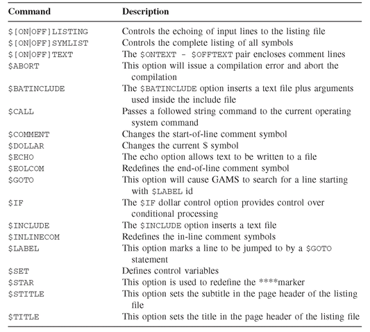
$ (dollar sign): Indicates a compiler directive or option. A list of the most common $-controls is given in Table 1.1. Many more exist than can be covered here; consult the User’s Guide (see Notes and References at end of chapter) for complete information.
Table 1.1: The most common $-control commands. See Section 1.3.10 for examples of the use of $SET, $IF, $LABEL and $GOTO for conditional compilation.
Any other character indicates a model source line. Customarily such lines start with a space character.
The main lexical elements of a GAMS statement are keywords, identifiers, and operators. The example model shows keywords in all capital letters, and identifiers use a mixture of upper and lower case, but the language is not case sensitive. Identifiers consist of letters, digits, or the underscore character, “-”, and must begin with a letter (in early versions of GAMS, identifiers were limited to at most 10 characters).
The GAMS examples that follow use comments of the standard kind (“*” in position 1), but in addition assume that text that starts with the sequence “#” to the end of the current line is regarded as a comment. Hence, the command is assumed to be in effect in all examples. C++ and Java programmers might prefer to use the more familiar
1.3.2 Sets
The primary tool for structuring large-scale models is the set. In any nontrivial model we will need to use data, variables, and constraints that are indexed, and sets form the basis for such indexing.
The simplest set declarations have the form: These lines declare the two sets Time and Bonds. The set Time contains the elements from 2002 through 2006 (the asterisk indicates filling out the intervening elements; one could have written this: SET Time /2002, 2003, 2004, 2005, 2006/;). Similarly, the Bonds set contains bonds named GOVT_1 through GOVT_4.
The ALIAS statement is a convenient way to declare indices to be used in connection with sets. The code above binds the name t to the set Time, and the names i and j to the set Bonds. These names can henceforth be used as indices into their associated sets (and only those sets).
The text “Bonds universe” in the Bonds declaration is an explanatory text that GAMS outputs in the listing whenever it lists the Bonds set, as a help in documentation. Such texts can occur in all declarations and can be a great help when reading GAMS listings. They need not be enclosed in quotation marks, but if they aren’t then they cannot contain certain characters, which can lead to quite subtle syntax errors.
Indices and indexation
Most GAMS modeling elements (data, variables, etc.) can be indexed, with up to 10 indices. For instance, a two-dimensional parameter F can be defined over the sets declared above as (more on data declarations in Section 2.2.1): These two declarations have identical meaning, given the ALIAS declarations of i and t, and specify that F takes two indices belonging to (aliased to) the sets Bonds and Time, respectively.

Indices are used, for instance in expressions, to pick out individual elements of indexed objects. If F(t,i) is a bond’s cashflows, then the following calculates each bond’s total cashflows: and stores it into the declared one-dimensional parameter. Notice that this assignment is automatically performed for each value i in Bonds. There is more information on the summation operation in Section 1.3.3.
Leads and lags are indices that are shifted by some constant, as in F(i,t+1) or F(i,t-1), respectively. The lead or lag need not be 1, but may be any integral expression whose value is known at compile time (endogenous). Leads and lags may only be used on static sets (not dynamic sets; see below).
There are no “index errors” in GAMS: If a lead or lagged index reaches beyond the underlying set, the result is 0; F(i,t+1) is 0 when t is the set’s last element.
It is sometimes convenient to treat sets as being circular, so that leads beyond the end “wrap around” to the beginning and vice versa. This is indicated by using the ++ or verb operator: F(i++1,t) references the next bond (from i), cyclically.
Constant set elements used as indices have to be specified in quotes:
The ORD and CARD set functions
The ORD function takes as an argument the name of a set (or an index aliased to a set) and returns the ordinate value of the index relative to the set. The CARD function takes a set name (or index) and returns the cardinality of the set, i.e., the number of elements in the set:

ORD is defined only on static, one-dimensional sets. They are not defined on constant set elements: ORD(“GOVT_4”) is illegal.
Subsets and multidimensional sets
A set can be declared as a subset of another set. For instance, specifies a subset, Callable, of the Bonds set and declares bonds GOVT_1 and GOVT_3 as being callable bonds. Subsets can be multidimensional:
  might specify the maturity years of the bonds as a subset of the cartesian product Bonds × Time. Note the dot-notation: GOVT_1.2003 specifies that the element (GOVT_1, 2003) belongs to Matur.

Dynamic sets
The sets seen so far were all static. Their elements were explicitly listed as part of their declaration. GAMS also allows dynamic sets, which are calculated during execution of the model allowing them to change dynamically depending on some model characteristics. Dynamic sets are always subsets of another set (or other sets) and do not have the / . . . / part in their declaration. Consider: This fragment defines the set Sub as a dynamic subset of Time, and initializes it to contain all but the first element. The expression YES $ (tau(t) >= 1) means to include element t in Sub if the condition following the $-operator is satisfied (conditional expressions are covered in detail in Section 1.3.3).

The ORD function is not defined on dynamic sets, but notice that a parameter such as tau, which is declared on the static set Time, can be used with both constant arguments, tau(“2006”) and with a dynamic set index, tau(Sub) or tau(s), as long as all arguments belong to Time. This is a very useful technique to extend ORD-like mappings from dynamic, even multi-dimensional, sets to numbers. CARD, however, is defined on dynamic (even multidimensional) sets.
1.3.3 Expressions, functions, and operators
Data manipulations and constraint definitions require the use of expressions and assignments. GAMS provides a rich set of operators and built-in functions for forming expressions. Expressions are built up from numerical values, that is, floating point constants, scalars, and parameter and table elements. Numerical values may be joined using operators; a list of operators is given in Table 1.2. GAMS also defines a number of functions; see Table 1.3. In addition, GAMS has a number of calendar (date/time) functions; see Table 1.4.
Table 1.2: Operators in GAMS expressions, grouped by priority. All operators accept and return numerical values. The logical operators interpret non-zero as true, and they return 0 or 1 for false or true.

Consider this simple example where some statistics of stock returns are calculated: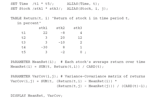

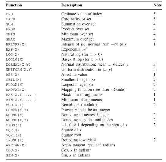
Table 1.3: Functions in GAMS. Notes: (1) non-differentiable and results in discontinuous nonlinear programming model if used on (endogenous) variables; (2) not continuous and illegal when used on (endogenous) variables; (3) pseudo-random, may not occur in equation definitions; (4) takes one or more set indices as their first parameter and perform an indexed operation; (5) takes a set or index argument.
The first assignment statement assigns to MeanRet(i) the average return of the three stocks over the five time periods. GAMS automatically performs the assignment for each value of the index i; notice the use of the SUM function to perform the summation over the t index, and the use of the CARD function to average.
The $-operator and conditional expressions
The $-operator is somewhat unusual and deserves special attention. It is a binary operator, and the meaning of the expression (exp) $ (cond) is as follows.
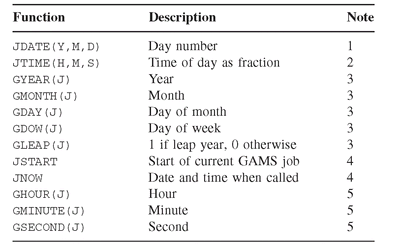
Table 1.4: Date and Time functions in GAMS. Notes: (1) JDATE converts a date (given as year, month, day) into the day number, where “Day 1” is January 1, 1900; (2) JTIME converts a time (given as hour [0, . . ., 23], minute [0, . . ., 59], second [0, . . ., 59]) into a fraction of a day; (3) these routines convert a day number into year, month, day, day of week, and check for leap years; (4) JSTART and JNOW return, in addition to date information, information on the time of day, taking no parameters; (5) these routines convert the result of JTIME, JSTART or JNOW back into time of day.
First, evaluate the expression cond. If its value is non-zero, then the complete expression has the value of exp, otherwise it has the value 0 and exp is not evaluated. For example, the annual cashflows of a set of bonds given their coupon rates and maturity years can be calculated by: where tau(t) maps elements of the time set to calendar years; a bond’s cashflow is composed of its price (negative at purchase), its principal payment (1, at maturity), and coupon payments; see Figures 2.1 and 2.2 for the complete model.

An expression such as tau(t) = 0 is called a conditional expression. GAMS has very simple rules for forming and using conditional expressions: any non-zero numerical value is interpreted as “true” when used in a conditional expression, and zero is interpreted as “false.” Consistent with this, the relational operators ( = , <, <= , >, >= , < >) and the logical operators AND, OR, and NOT return the numerical values 1 for “true” and 0 for “false.” It is advisable to use parentheses around the operands of the $-operator; this aids readability and avoids any confusion about the priority of $ relative to other operators.
Notice also the use of an indexed set or parameter as a condition. Given the declarations the expressions Matur(i,t) and F(t,i) are legal $-conditions, testing whether the pair (i,t) belongs to Matur, or whether F(t,i) is non-zero, respectively.
The $-operator also has another important function as a control structure: any time GAMS performs an indexed operation, a $-condition can be used to specify a subset of the indices over which the operation should be performed. Details are given in the relevant sections under equation definitions (Section 1.3.6), assignment statements (Section 1.3.4), and the SUM, PROD, SMIN and SMAX functions below.
Special functions: SUM, PROD, SMIN, SMAX
The functions SUM, PROD, SMAX, and SMIN have two arguments where the first must be a set (or index) expression. They form the sum, product, element-wise maximum, and element-wise minimum over the second argument values: Note the use of parentheses to sum over multiple indices.
The index set over which the operation is applied can be qualified using the $-operator, as in: The operation will be performed only over indices that satisfy the condition. When the condition is simply an indexed set or parameter, as in Callable(i), the conditional summation can be abbreviated as shown in the second line above, which aids readability.

Applying one of these functions over an empty set results in the operations’s neutral element: 0 for SUM, 1 for PROD, -INF for SMAX, and INF for SMIN. Comparing index values directly is not possible: It is necessary to use some function that converts from set elements to numerical values, such as ORD or some parameter indexed by the set (as tau in the example above). For the special case of testing for equality, however, GAMS has a function SAMEAS:
  SAMEAS compares the names of the set elements referred to by the indices (not their ordinal values), and is legal even if the two indices belong to different sets.

Extended arithmetic: INF, EPS, NA, UNDF
GAMS defines certain special values that can be used in and result from expressions, but which are not numbers. The most common one is INF, which represents the (extended real) number ∞. For instance, a free VARIABLE has lower and upper bounds -INF and INF.
Another common special value is EPS, which is returned by solvers as the marginal value of degenerate variables or constraints (that is, non-basic variables or binding constraints with zero marginals). Knowing this makes it easy to pick out the final basis from a linear programming solution as those variables and (slack/artificial variables corresponding to) equations having “.” as the marginal value as opposed to EPS or a non-zero value.
Finally, the last two special values are NA (used to represent missing, or “Not Available,” data) and UNDF, for undefined (usually erroneous) results.
The rules for arithmetic using these values are well defined in GAMS but rather complicated; see the User’s Guide or the library model crazy.gms for details.
1.3.4 Assignment statements
The assignment statement is used, as in any other language, to assign values to parameters (SCALARs, PARAMETERs, and TABLEs). The parameter on the left-hand side always has all indices specified, and GAMS automatically performs the assignment for each index value. Some examples: The first line is a simple assignment of a single value. The second is performed for all indices i, the third only for those values of i that satisfy the condition. Note that in a conditional assignment that the condition is placed before the = sign.

Assignments performed over indices are performed in “parallel,” in the sense that the right-hand side is first calculated for each index value, and only then is the left-hand side simultaneously updated. See in Section 1.3.9 (the LOOP statement) how this behavior can be circumvented if desired.
As a complete example, consider the following calculation of a lower-triangular matrix to hold covariance information:
 In this example we want to calculate variance-covariance information into a matrix efficiently, by only storing elements in the lower triangular half of the VarCov2 matrix, defined by the dynamically calculated subset SET Lower. The assignment to VarCov2(i,i)) calculates the diagonal, and the assignment to VarCov2(Lower(i,j)) is shorthand for:
 so that only below-diagonal elements are assigned. Altogether, this calculation is almost twice as fast as calculating VarCov shown on page 7, yet used in a typical variance expression such as
 it is equivalent (but again about twice as fast to evaluate).


1.3.5 Variable declarations
Variable declarations are used to declare the variables used in a model. Variables can be continuous or discrete or some mixture of the two. Continuous variables are allowed to take on a range of variables between some (possibly infinite) lower and upper bounds, while discrete variables must take on an integer value between some finite bounds. The different declaration possibilities are shown in Table 1.5. Variables can have up to 10 indices.
Variable attributes
After declaration of a variable it is always possible to change its bounds:
 Here, a two-dimensional array of variables is declared as non-negative (default bounds 0 and ∞), but then the bounds are reset to -4 and 10, by setting LO and UP attributes. Finally, y(“2”,”3”) is fixed at a specific value. Assigning a value to the FX attribute is equivalent to setting the variable’s lower and upper bounds to the same value. Fixing a variable does not remove it from the model; see the HOLDFIXED attribute on page 15 for how to do this. Variables also have two other attributes which are set by solvers: L is the “level” value (for instance the optimal value after the problem is solved), and M is the “marginal,” or reduced cost. These can both be initialized by the user, which is useful in nonlinear programming to provide a starting point for the solver.

Table 1.5: The different kinds of variables and their declaration. The default bounds can be reset through the LO and UP (or FX) attributes.

Variables also have a scaling attribute, SCALE; see the User’s Guide for details.
1.3.6 Constraints: Equation declarations
Equations are used to declare and define model constraints: Here, we declare a set of constraints constr(i), and an individual constraint, objective. They are then defined (indicated by the “..” symbol). Each of the constraints constr(i) is a less-or-equal inequality constraint, as indicated by =L=. The objective constraint is an equality indicated by =E=. Greater-or-equal constraints are specified using =G=. A fourth relation, =N=, indicates that the constraint is present but non-binding; no use has yet been found for it. The expressions used to define constraints are covered in Section 1.3.3.

Endogenous variables in constraints
Constraint expressions are the only places where endogenous variables (GAMS variables), like x(j), can be used without their attributes (L, M, UP, LO, etc.). Note a few cautions regarding endogenous variables in constraints (an “endogenous expression” is an expression that is or contains an endogenous variable):
• nonlinear GAMS functions or operators, when used on endogenous expressions, lead to nonlinear (NLP or DNLP) models; see Section 1.3.8 for details on model types.
• non-continuous GAMS functions may not be used on endogenous expressions.
• the pseudo-random number generator functions UNIFORM and NORMAL may not be used at all in constraints.
• endogenous expressions cannot be used in the conditional part of a $-condition.
A $-condition may be placed before the .. symbol in a constraint definition. The constraint is only then generated and included in the model if the condition is satisfied:

Equation attributes
Constraints have the attributes LO, UP, L and M. To understand these it is useful to consider, for instance, a less-equal constraint to be written as: where lhs consists of all variable terms of the constraint and rhs consists of all constant terms. Then the level attribute .L is the value (after a solve) of the constraint’s left-hand side, and the bounds attributes LO, UP are the bounds on it; for a less-equal constraint the left-hand side has bounds -INF and rhs. The M attribute is the constraint’s dual price.
1.3.7 Model declarations
Model declarations serve to collect the constraints and variables that are part of the model, and to name the model.
Between the slashes are listed the names (without indices) of any constraints that should be part of the model Dedication. If all the constraints defined in the source file up to this point are part of the model, one can write:
Model attributes
Models have “attributes” which are used to communicate information to and from a solver. Some are set by the user and correspond to setting the corresponding value using an OPTION statement; see Table 1.6. For instance, Dedication.RESLIM = 200; allows the solver to spend at most 200 seconds solving the Dedication model.
Others are set as a result of executing a SOLVE statement and they can be used to test the result of solving a model and hence decide on further actions to take:
 The most important values of MODELSTAT are 1: optimal, 2: locally optimal, 3: unbounded, and 4: infeasible;
Table 1.6: The most important OPTIONs. The argument N indicates a non-negative integer.


Substituting fixed variables
The variable suffix FX will “fix” a variable, i.e., set its upper and lower bounds to the same value, but the variable is still present in the problem even though it has only a single feasible value. The MODEL attribute HOLDFIXED, when set to 1: will cause the values of all fixed variables to be substituted for the value throughout in the model. This can greatly reduce the complexity of a model, for instance converting a nonlinear model to a linear one. The only piece of information lost is the variable’s dual information (marginal).

1.3.8 The SOLVE statement and model types
The SOLVE statement has the general form: where model_name is the model to be solved, obj_var is the variable whose value should be minimized (one can also ask for MAXIMIZING the value), and model_type indicates the type of model to be solved; see Table 1.7. GAMS will select a default solver that is capable of solving the indicated model type, or a desired solver can be specified:
 causes GAMS to use BDMLP to solve LP models.
The variable obj_var appearing in the SOLVE statement should be continuous without bounds.
Model types
GAMS recognizes several model types, as listed in Table 1.7. The most important are:
• LP: If the model contains only linear constraints and continuous variables, it’s an LP. LP’s are generally very easy to solve, except when extremely large.
• MIP: If the model contains linear constraints but discrete (integer or binary) variables, then it’s a MIP model. These can be very time-consuming to solve. Be aware that
INTEGER VARIABLES have implicit upper bounds of 100, so it is usually a good idea to set relevant upper bounds explicitly. Also, by default, a solution that is probably within 10 % of the optimum may be returned - to force the solver to go for an optimal one use OPTION OPTCR = 0. Also, the default iteration and resource limits of 1000 iterations and 1000 CPU seconds are, in some cases, not sufficient for the convergence of the solver. Use, for instance, OPTION ITERLIM = 999999999, RESLIM = 1200; to allow 20 minutes but virtually unlimited iterations for the solution.
• RMIP: To solve a MIP model while ignoring the integrality constraints, use RMIP. This is useful for model debugging.
• NLP: If your model contains nonlinear constraints and continuous variables, it’s an NLP. These can be easy or difficult depending (mostly) upon whether the constraint set is convex, and the objective function convex (for minimization) or concave (for maximization). The best result possible for an NLP is “locally optimal”; the solver has no way to guarantee that a locally optimal solution is also globally optimal.
• MINLP: May contain nonlinear expressions and discrete variables.
• DNLP: May contain nonlinear constraints that are not differentiable, hence very unreliable to solve. One should usually try to reformulate such models, or “smooth” any “kinks.”
Table 1.7: GAMS Model types.

1.3.9 Control structures
The control structures consist of the IF, WHILE, FOR, LOOP statements. They are used to control the execution of statements, depending on a condition. Control statements may not contain declarations.
The IF statement
The IF statement has the following forms: where condition is a conditional expression (1.3.3) and stat-seq is a semicolon-separated list of executable statements. Some examples follow:
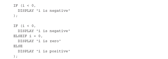 The IF . . . ELSEIF . . . variant allows an arbitrary number of ELSEIF parts, and the ELSE part is optional.


Iterative control structures
These statements allow repeated execution of groups of statements until some condition is satisfied (WHILE), or under control of either a scalar parameter (FOR) or a set index (LOOP). Their syntax is: where condition is a conditional expression (1.3.3) and stat-seq is a semicolon-separated list of executable statements. The FOR loop iterates a parameter parm through a range of values, as for instance:


A powerful use of the iterative statements is to solve sequences of related models by having a SOLVE statement in the iteration. To use this facility it is necessary to know that every time a SOLVE statement is executed, the model is regenerated from scratch: GAMS runs through the equation definitions using the latest values of all sets and parameters they reference. By changing these as part of the iteration one can generate a different model in each run through the loop.
As an example, Figure 1.1 shows how to solve a sequence of related models under control of a FOR statement. The model is the Klee-Minty model (see, e.g., Nash and Sofer [1996] for a discussion on the Klee-Minty problem), which is interesting because it may require 2m iterations with a naive implementation of the simplex algorithm, where m, the number of variables and constraints, is a parameter:


(1.4)

(1.5)

(1.6)
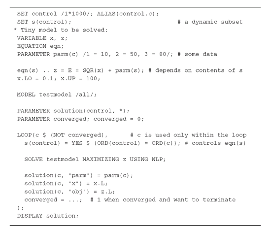
As another example, Figure 1.2 shows the use of a LOOP to control the iterations, and a dynamic set s is used to control generation of the model. A solution report is built along the way.
Figure 1.1: GAMS model for solving the Klee-Minty problem for m = 1, 2, 3, 4.
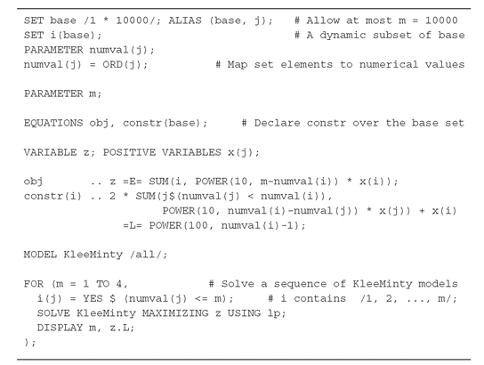
Figure 1.2: Using a LOOP iterative statement to control a SOLVE statement and to create an iteration-by-iteration solution report. Notice the way the three sets/indices (control, s, and c) are declared and used: control is the base set, allowing up to 1000 iterations; c is the loop control index; and s is a dynamic subset of the control set, which (in this example) contains the the current loop index as its only element, and which in turn controls the generation of equation eqn. The loop can be terminated at any time by setting converged to 1.
Defeating parallel assignment
An assignment statement such as is executed “in parallel”: GAMS performs the assignment for each value of the controlling index i “at once.” But sometimes the parallel assignment feature gets in the way. Consider calculating the Fibonacci numbers from 1 to 100. One might be tempted to do this:


The last assignment would not work because of the “parallel assignment” feature of GAMS: Most of the values referenced on the right-hand side are equal to zero (i.e., =Fibonacci(“3”) through Fibonacci(”100”)), and the values assigned to Fibonacci(“1”) through Fibonacci(”2”) use undefined indices, -1 and 0. The way to implement this kind of recurrence relation is to force GAMS to execute the assignment element-by-element in a specified order, rather than in parallel. The LOOP statement does this:

Note the use of the $-operator to limit the LOOP statement to values of i greater than 2.
1.3.10 Conditional compilation
Some of the GAMS $-control commands (see Table 1.1) are particularly useful for conditional compilation, that is, including or excluding parts of the GAMS source code depending on some condition. We give here an example:

1.4 Getting Started
The GAMS system can be executed in two modes. On computers running Windows, through an Integrated Development Environment graphical interface that facilitates managing the files involved in a GAMS project. On computers running Unix, through a simpler command-line interface where the GAMS system is called from a command-line window. Both modes of execution are described below.
1.4.1 The Integrated Development Environment
The GAMS Integrated Development Environment (IDE) provides an environment for managing GAMS modeling projects that facilitates the process of editing input files, executing GAMS, and viewing output files. It is a graphical environment that is available on Windows systems, and is expected to be available on Unix systems as well.
The GAMS IDE is project-oriented. This means that all the files associated with a model, or a set of models, are collected in a project file. Even if your GAMS “project” consists of only a single GAMS input file and its output file, there are advantages to organizing these files in a project.
Creating a new GAMS project
To create a new GAMS project, first close any open files in the GAMS IDE (“File - Close” for each one). Then open the “File - Project - New Project” window and navigate to the directory where you want your project to reside (you may already have your GAMS source file there). Under “File name,” enter the name of your project. To add existing source files to your project, use “File - Open” and navigate to your source files (usually .gms and .inc files), adding them to the project one by one (or add multiple files at once, using the standard key sequences). To create a new source file in your project, use “File - New”; then immediately after “File - Save as” to give the new file a name.
Opening an existing GAMS project
Use “File - Project”, to check if the project is already listed in the window, or click “Open project” and navigate to it.
Executing GAMS models
To execute a GAMS source (.gms) file, make sure it is the active file in the IDE (“has focus”). Then use the Run entry from the File menu, press F9 or click on the Run icon at the top of the main window. Next to the Run icon is an entry field to specify additional parameters for the GAMS run. Additional parameters have the same effect as if they were specified from the commandline.
While GAMS is compiling and executing the model it displays a log window showing what is going on. If the run takes a while, you may check the Update entry at the bottom to make sure the log window is updated every time GAMS or one of the solvers outputs a line. After execution, the listing file is made the active file, and can be examined for the solution or any error messages.
1.4.2 Command line interaction
The simplest and most general way to use the GAMS system is from the command line through text files. An input file containing the model’s source code, and having a name with the extension .gms, is created using an ordinary text editor, such as vi, emacs, or Notepad (if using a word processor you should “save as type .TXT”). This file is then submitted to the GAMS system by issuing the command: from the Unix prompt. GAMS will look for and compile the file dedicate.gms, and generate an output file, dedicate.lst, containing a listing of the input file and the solutions of any models solved. This file is then examined using a text editor. It is often convenient to have several open windows: one in which to edit the input file, one to call GAMS, and one to look at the output.
1.4.3 The model library
The fastest way to build a new model, or to learn the language, is to study existing models that address a related problem. The GAMS system includes a large library of models that demonstrate applications drawn from engineering, finance, and economics. The library is an excellent resource for learning GAMS, or for learning about modeling in a particular problem area. The FINLIB library, which is documented in this book, contains several of the financial optimization models discussed in the companion volume Practical Financial Optimization.
From the GAMS IDE, “File - Model Library - Open GAMS Model Library” gives access to more than 100 models in the standard library and to the FINLIB library. Clicking on one of the models will add it to your current project and you can now modify it as you want (you will not be allowed to modify the original file).
From the command line, copies a file containing a list of the library models into the current directory; the commands
 both copy model number 1, dedicate.gms, into the current directory.
Notes and References
The GAMS manual, GAMS: A User’s Guide and other documents can be downloaded from http://www.gams.com. A demonstration version of the GAMS system can be obtained from http://www.gams.com/download.
At the time of writing it is also possible to download the GAMS Integrated Developer Environment (for Windows), containing a sample of solvers and the GAMS main compiler. This system runs in “demo mode,” allowing the solution of small to medium-sized models. To obtain licenses for solving larger models, for other solvers, or for systems for other machines, contact [email protected].
..................Content has been hidden....................
You can't read the all page of ebook, please click here login for view all page.
