Chapter 5
Scenario Optimization
5.1 Preview
In this chapter we develop the GAMS models for scenario-based portfolio optimization. The development is based on the discussion of Chapter PFO-5. The following models are discussed in this chapter and the GAMS source code for each is given in the associated FINLIB files:
Mean absolute deviation (MAD) models are based on Section PFO-5.3. We give models which select a portfolio by minimizing the mean absolute deviation from a reference point or a target liability. We also provide a tracking model where the target is a market index.
• MAD.gms
• TrackingMAD.gms
Regret models are based on Section PFO-5.4. In this case the risk function is measured in terms of negative deviations from a benchmark; we also use the model to highlight the differences with MAD tracking models.
• Regret.gms
Conditional Value-at-Risk (CVaR) models are based on Section PFO-5.5 and optimize CVaR, which has the nice property of being a coherent risk measure.
• CVaR.gms
Expected utility maximization models are based on Section PFO-5.6 and maximize the expected value of investors’ utility.
• Utility.gms
Put/call efficient frontier models are based on Section PFO-5.7. We build put/call efficient frontiers and show the effects of liquidity constraints.
• PutCall.gms
5.2 Data sets
The GAMS models of this chapter are set up using three common data sets. As far as possible identical data are used in setting up the models so that users can compare and contrast the results. The data sets are given in the following files:
• Corporate.inc, contains simulated return data for 17 bonds and a risk-free asset, for 1000 scenarios.
• WorldIndices.inc, contains 10-year monthly return data for 13 asset classes, including several stock and bond indices from the international markets for 120 scenarios.
• Index.inc, contains 10-year monthly return data of an index constructed by averaging the returns of the 13 asset classes in WorldIndices.inc.
The models implemented in this section are designed in such a way that it is irrelevant if they are based on a view of the scenarios using forward-looking simulations, or if they use samples from historical time series. Scenario generation methods are described in Chapter PFO-9, and here we take the scenario data as given input.
The data files used by the models are controlled by the GAMS INCLUDE command:

The data files contain simple two-dimensional data, corresponding to asset returns for each scenario. As an example we show here a fragment of Corporates.inc: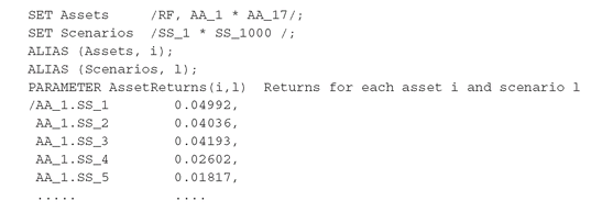 The data structure is consistent with a single-period model, as opposed to the multi-period models we will develop in the next chapter. Furthermore, the use of aliases allows us to build GAMS models that are quite general and can be run with different data sets. In other words, it is not the name of the set, but the names of the aliases that will be used in the model equations.

5.2.1 The FINLIB files
The GAMS data for the models of this section are given in the following files:
• WorldIndices.inc
• Corporate.inc
• Index.inc
5.3 Mean Absolute Deviation Models
We develop in this section some variants of the mean absolute deviation (MAD) models, Model PFO-5.3.1 (MAD.gms) and Model PFO-5.3.5 (TrackingMAD.gms). We start from the general MAD minimization model and we repeated it here:
Note that the model is defined here using asset values (or prices) whereas the scenario data are asset returns. Hence, the model implemented in GAMS uses the value of one unit invested in an asset. Without loss of generality, we also assume that the initial prices (P0i) are all equal to 1.
The annualized returns are stored in the parameter AssetReturns(i,l) denoting the return of asset i in scenario l. The decision variables are x(i), the holdings in stock i. Note that these are not fractions of total holdings as was the case in the mean-variance model, but are expressed in face value and are constrained by a given nominal budget.

In this model, the scenarios are considered to be equally likely, and their probabilities are declared and initialized as follows: Note that, since we are using a large number of scenarios, the above assumption is not restrictive. We are treating our sample as a statistical sample drawn from a given population or distribution function, and the larger the number of scenarios, the better is the approximation of the underlying distribution.

To calculate the mean absolute deviation of the portfolio, we first need to keep track of the values of each asset in each scenario, P(i,l). We also compute and store in EP(l) the expected value of each security.
These are defined in GAMS as: The mean absolute deviation is defined by the scenario-dependent variables y(l). They measure the absolute deviation of the portfolio, under each scenario, from its expected value (see Equations PFO-5.25-PFO-5.26). The corresponding equations in GAMS are given as follow:
 The objective function is defined as the average, over all scenarios, of the deviations y(l); this is an estimate of the portfolio mean absolute deviation.


To build the efficient frontier of MAD vs expected return, we minimize the MAD objective function and constrain our portfolio to have an expected value greater or equal to a given target return (MU_TARGET). We do this in a FOR loop where the target return is increased from the lowest to the highest attainable expected return:


The model shown weighs over- and under-performance equally. Model PFO-5.3.3 shows how to differentially penalize downside from upside deviations:


Model PFO-5.3.3 Upside potential and downside risk in mean absolute deviation
(5.7)
(5.8)
(5.9)
(5.10)
(5.11)
(5.12)
We rework the related GAMS equations as follows: where lambdaPos and lambdaNeg are suitably declared weights.

As shown in Section PFO-5.3.2, when the deviation is measured with respect to the expected value of the portfolios, Model PFO-5.3.3 is equivalent to Model PFO-5.3.1. This is demonstrated by the results obtained from running the two models and inspecting the portfolios for each target returns.
5.3.1 Downside risk and tracking models
In TrackingMAD.gms we deal with models exploiting the MAD feature of penalizing differently downside from upside risk. We are interested in placing a limit on shortfalls with respect to the portfolio expected value or to a given target. The target could be stochastic and, if the target is a market index, the model is also known as a tracking model, yielding a tracking portfolio.
Given a user-specified tolerance, ε, the portfolio that maximizes the expected return, and places a limit on deviation below the portfolio expected value, is given in Model PFO-5.3.4:


 However, instead of solving Model PFO-5.3.4 for a specific tolerance, it is preferable to build an efficient frontier to trade-off the downside error against the expected return. The larger the value of the allowed shortfall, the higher the expected return attainable. Investors will decide the acceptable deviations from the target, but consistency with the goal of tracking an index dictates that ε should be made as small as possible.
Model PFO-5.3.4 Portfolio optimization with limits on maximum downside risk
(5.13)
(5.15)

(5.16)
To implement this model, we declare the scalar EpsTolerance and set it to a high value; EpsTolerance is then reduced for as long as the model yields a feasible solution. We use the GAMS WHILE statement to solve recursively Model PFO-5.3.4, and check for infeasibility from the status returned by the model extension MODELSTAT.
The main changes with respect to MAD.gms are reported here: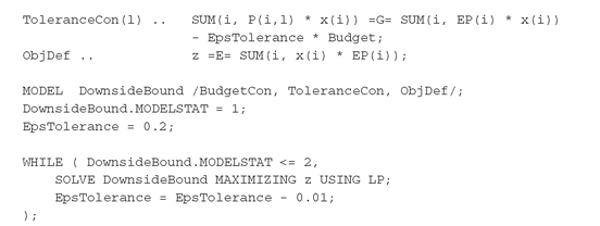

If the model terminates with an optimal or locally optimal solution, then the model name extension MODELSTAT returns 1 or 2 and the WHILE loop is continued. If the model is infeasible, the value 4 is returned and the loop terminates.
Extending Model PFO-5.3.4 to tracking a constant target, or a stochastic index, is straightforward. We simply replace the expected value in equation (5.14) with the desired target g, or with the index values under each scenario gl : 


Model PFO-5.3.5 Tracking model
(5.17)
(5.18)
(5.19)
(5.20)
In TrackingMAD.gms we modify the ToleranceCon(l) equations to take into account the constant target portfolio return or the market index. Note that both targets must be consistent with the scenario used. There is no hope of attaining a monthly 10 % target when the assets used return an average 3 % per month; indeed, the model will yield a feasible solution only for large downside deviations.
The example in TrackingMAD.gms is set up using the WorldIndices.inc data. We select a fixed target equal to 2 %, and include a target index (Index.inc) obtained as a simple average of the 13 assets contained in WorldIndices.inc. Note that if we set the tolerance equal to zero the model produces a portfolio with holdings in each asset identical to the composition of the equally weighted target index. Of course, this portfolio is of no practical use as the transaction costs and the managing costs will deplete the performance.
The main changes in the GAMS code are reported here: In Figure 5.1 we display the trade-off between tolerance and expected return. The tolerance is given in absolute value (EpsTolerance * Budget), and is computed for different fixed-target portfolio returns (TargetIndex(l) = K). For TargetIndex(l) = 0.10 (10 % of the budget), the efficient frontier is made up by very few points. This occurs because the expected returns of the assets available range between 0.2 % to 1.3 %, and therefore, it is very difficult to achieve the 10 % target unless a high tolerance is allowed, which of course means that the target is not met.

5.3.2 Comparing mean-variance and mean absolute deviation
We now compare the results of the mean-variance optimization model (MV) from Section 3.2, to the results of minimizing the mean absolute deviation (MAD). For a given target expected return, the MAD model minimizes the portfolio mean absolute deviation around its expected return, while the mean-variance model minimizes the variance of the portfolio return.
Figure 5.1: Tolerance (in absolute value) vs expected return for a fixed target equal to 2%, 5%, and 10%. Higher target returns are difficult to meet, producing a more restricted efficient frontier.

According to Theorem PFO-2.3.2, the MAD and variance of a portfolio are closely related, provided the asset universe has multivariate normally distributed returns. The relation between the MAD w(x) and the variance σ (x) is given by:
 This means that MV and MAD models, for identical target returns, will return similar portfolios, and that the MAD and the variance values of those portfolios will satisfy equation (5.21).

We can easily verify this observation using both data sets provided. The details of the implementation are given in MAD.gms. We first calculated the mean and the variance-covariance matrix of the asset returns from the given scenario data to solve the MV model, and then solved the MAD model using directly the scenario data for each level of the target return. The results are stored in MADvsMV.csv.
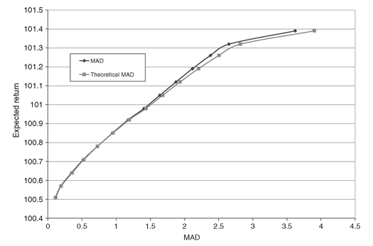
In Figure 5.2 we show the efficient frontier obtained with the MAD model and its counterpart using equation (5.21).
Note that the two curves mostly overlap and are only slightly different for the high-risk portfolios. The difference is attributed to the fact that the returns from our sample data are only approximately normally distributed due to the small sample size. This, together with the fat tails that characterize the stock market returns in our data, cause violations of the formula given in (5.21). The results in this figure imply that the portfolios obtained with the two models should be similar.
Figure 5.2: MAD efficient frontier and MAD vs expected return for the mean-variance efficient portfolios as given by equation (5.21). The two frontiers are identical, within numerical errors, confirming the relation between MAD and variance.
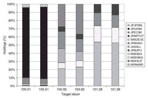
Indeed, in Figure 5.3 we show a sample of portfolios with the same target expected return. We observe that the asset allocations are fairly similar and their differences are negligible. This has practical significance because it means that MAD, which is a linear programming model, can be used instead of the more difficult, quadratic mean-variance model. Of course, this can be appreciated for large-scale models with thousands of variables. Furthermore, as variance and covariance data are usually estimated from historical data (i.e., scenarios) these can be used directly by MAD, bypassing the variance/covariance calculations.
5.3.3 The FINLIB files
The GAMS source code and data for the models of this section are given in the following files:
• MAD.gms
• TrackingMAD.gms
Figure 5.3: Portfolios obtained by solving the MAD and MV model for the same level of the target return. MV and MAD models yield the same portfolio when the return distribution is multivariate normal. Deviations are due to fat tails or small sample size.
5.4 Regret Models
The model to minimize expected regret, Model PFO-5.4.1, is similar to the MAD models of the previous section and is repeated here:
Indeed, by setting λu = 0, λd = 1, and gl = V (x, ), we obtain Model PFO-5.3.3.
A different formulation of the regret model allows deviations from the target up to a given threshold εV0. We give here the formulation of the ε-regret Model PFO-5.4.3, where, instead of minimizing the expected regret, we constrain the expected regret while maximizing the expected return:


Model PFO-5.4.3 Portfolio optimization with ε-regret constraints
(5.28)
(5.29)
(5.30)
(5.31)
(5.32)
(5.33)
We observe that if we set ω = 0, Model PFO-5.4.3 is equivalent to the tracking model Model PFO-5.3.5, and the ε-regret models generalize tracking models.
We implement Models PFO-5.4.1 and PFO-5.4.3 in two variants. Namely, we first maximize the expected return, while placing a bound on the expected regret, and then minimize the expected regret while requiring the expected return to be greater than a given target. Of course, both formulations, with and without the ε-regret, will deliver the same efficient frontier. The main equations and statements are displayed here: To run Model PFO-5.4.3, simply replace RegretCon with EpsRegretCon in the MODEL statements.

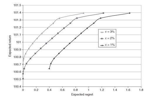
In Figure 5.4 we show the efficient frontiers for ε-regret 1%, 2%, and 3%, respectively. By increasing ε-regret the efficient frontier moves upward. This is also observed in Figure 5.1, where the efficient frontier is moved upward by lowering the target return. Indeed, adding the ε-regret tolerance is equivalent to reducing the target return gl.
We point out that the efficient frontiers displayed in Figure 5.1 and 5.4 are plotted together for convenience. In other words, the efficient frontiers further up in the graph do not dominate those below, in the usual sense of efficient frontiers, since the portfolios also differ in the target liability (Figure 5.1), or in the maximum allowable regret (Figure 5.4).
Figure 5.4: ε-regret efficient frontiers obtained with ε equal to 1%, 2%, and 3%. By increasingthe ε-regret parameter, the efficient frontier is pushed further up.
5.4.1 The FINLIB files
The GAMS source code and data for the models of this section are given in the following files:
• Regret.gms
5.5 Conditional Value-at-Risk Models
The Value-at-Risk (VaR) concept defined in Section PFO-2.6 can be used to control the risk profile of portfolios and is considered an industry standard. However, VaR minimization leads to integer programming models that are very difficult to solve when the number of scenarios involved is high.
The notion of Conditional Value-at-Risk (CVaR) comes in handy when optimization is required (see Definition PFO-2.6.3). First, CVaR has the nice theoretical property of being a coherent measure as discussed in Section PFO-2.7. Furthermore, CVaR is a convex, smooth function of the portfolio composition, and if the loss function is linear and scenarios are given in discrete form, the CVaR formula is a linear function of the asset allocation, and hence we can optimize this risk measure using linear programming. Finally, since CVaR is always greater than VaR, minimization of CVaR also bounds VaR.
The minimization of Conditional Value-at-Risk (CVaR) is given in Model PFO-5.5.1, which is reproduced here:
The constraint structure of the CVaR model is similar to the MAD and regret models. In particular, equation (5.36) has the same form as the regret equation (5.24), and the MAD equations (5.3)-(5.4). Unlike those models, the variable ζ (which is the VaR value) plays the same role of a tolerance or regret, but it is also a variable of the optimization model itself.
Model PFO-5.5.1 is a linear model, provided the loss function L(x, Pl) is a linear function of the portfolio x, which is usually the case. In our setting we use three linear loss functions as follows:
• L(x; Pl) = V0 - V(x; Pl ), loss of the final portfolio value V(x; Pl ), with respect to the initial investment V0.
• L(x; P l ) = gl - V (x; P l ), loss with respect to a random target gl (or a fixed target, in case gl = g for all scenarios l ∈ Ω). A portfolio model with this loss function is also known as benchmark VaR.
• L(x; Pl) = V (x; ) - V (x; Pl), loss with respect to an endogenous target given by the expected value of the portfolio. In this case, if the returns are multivariate normal, the CVaR portfolio and the mean-variance portfolio will coincide; see Uryasev and Rockafellar (2000).
The linearity of the risk measure makes the CVaR model suitable for an alternative formulation, as was also done in the regret and the MAD models, whereby we maximize the expected return of the portfolio and restrict the level of the CVaR to be less or equal to a target risk ω. We reproduce the model with CVaR constraints in Model PFO-5.5.2.
Model PFO-5.5.2 Portfolio optimization with CVaR constraints
(5.40)
(5.41)
(5.42)
(5.43)
(5.44)
(5.45)
The GAMS code for both Models PFO-5.5.1 and PFO-5.5.2 can be found in CVaR.gms. The implementation uses the same approach adopted for the regret models, namely, we declared two equations that will compute, respectively, the CVaR and the expected return of the portfolio:
Using the dollar statement we declare in a single equation the three different loss functions, and the parameter LossFlag will switch to the desired definition.

Finally, CVaRCon and VaRDevCon(l) describe the CVaR constraints and the deviations from VaR for every scenario:

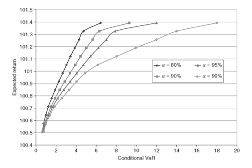
In Figure 5.5 we show the mean-CVaR efficient frontiers for different values of the confidence level α. Since a higher α implies that we are interested in more extreme losses, for the same level of the target return the expected CVaR is higher, and therefore the efficient frontiers are squeezed together toward the bottom.
5.5.1 The FINLIB files
The GAMS source code and data for the models of this section are given in the following files:
• CVaR.gms
Figure 5.5: CVaR efficient frontiers obtained by varying α. As α increases (80%, 90%, 95%, 99%), the efficient frontiers are pushed downwards, since for the same level of expected return a higher VaR of the losses distribution has to be selected.
5.6 Utility Maximization Models
Utility theory provides a theoretical framework for optimizing investor behavior when faced with uncertainty. The basic assumption in utility theory is that decision makers act, or should act, to maximize their expected utility and we implement models to do so based on Section PFO-5.6.
Letting p denote the stochastic return of a portfolio, and
 the return under scenario l in a scenario-based model, then the objective to maximize expected utility is:
 where U(·) is the utility function. The utility function must be monotonically increasing; a concave utility function is consistent with risk-averse behavior, while a convex utility function is consistent with risk-seeking behavior. A linear utility function implies risk-neutral behavior.
A class of utility functions often used in financial optimization are the isoelastic utility functions (Definition PFO-2.8.6), a special case of which is the growth optimal utility function (Definition PFO-2.8.7). They are parameterized by a risk parameter γ ≤ 1, whereby lower gamma values imply higher risk aversion, while γ = 1 denotes risk neutrality: The formal connection between the two branches of definition (5.46) is that the expression
 γ ((1 + r)γ - 1) converges (pointwise) to log(1 + r) for γ → 0.
(5.46)

We repeat here Model PFO-5.6.1 to maximize the expected utility:


Model PFO-5.6.1 Expected utility maximization
(5.47)
(5.48)
(5.49)
(5.50)
In Utility.gms we implement a slightly different version of Model PFO-5.6.1 which is consistent with the problem discussed in the application on insurance policies with guarantees (see Chapter PFO-12 and Section 8.4 later in this book). The model we implement is more general than Model PFO-5.6.1; in particular we assume that the decision maker has to allocate a given amount of equity among the available assets in order to maximize the expected utility of the return on equity (ROE). The ROE is given by the ratio between the final wealth provided by the portfolio and the initial equity invested:
(5.51)
We declare in GAMS the variables ROE(1) and use them as arguments of the utility function. (This is not really necessary, and the dimension of the model can be reduced by substituting the definition of the ROE directly in the objective function. However, readability is improved with the use of dummy variables.) To handle the case for γ = 0, we split ObjDef in two parts using the dollar statement: We solve ExpectedUtility for a sequence of risk aversion parameter, gamma, compute the certainty equivalent ROE CeROE, and store the correspondent portfolios in a file.

Figure 5.6: Risk aversion vs CeROE; the higher the risk aversion (i.e., large negative values of γ) the lower the CeROE.
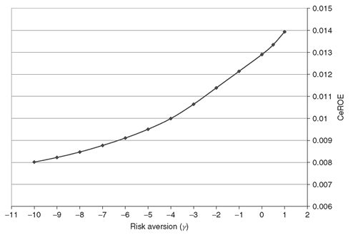
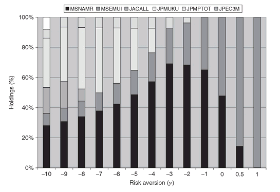
In Figure 5.6, we show the CeROE as a function of the risk aversion parameter gamma. As expected, the lower the gamma the higher the risk aversion, and therefore the lower the CeROE achieved. This occurs because risk-averse investors will prefer to allocate their equity on less risky assets. The latter, in general, have a lower expected return, thus lowering the final performance of the portfolio. In Figure 5.7, we display the portfolios obtained for different values of gamma. The risk-neutral investor (gamma = 1) will allocate the whole Equity on a single asset, while the risk-averse investors will diversify their investment among the available assets.
5.6.1 The FINLIB files
The GAMS source code and data for the models of this section are given in the following files:
• Utility.gms
5.7 Put/Call Efficient Frontier Models
Put/call models are analyzed in Section PFO-5.7.1. They provide a framework to select portfolios whose risk measure is given by the expected value of the downside deviations from a given target, and the reward measure is the expected value of the upside deviations from the same target. Put/call models also provide a valuable tool to determine the liquidity premium or discount with respect to prices under infinite liquidity.
Figure 5.7: Asset allocation for different levels of risk aversion. For higher risk aversion (i.e., large negative values of γ ) the asset allocation is more diversified.
We replicate here Model PFO-5.7.1 that generates unconstrained efficient put/call portfolios:


Model PFO-5.7.1 Put/call efficient portfolio
(5.52)
(5.53)
(5.54)
(5.55)
Note that Model PFO-5.7.1 is unconstrained and its dual formulation is given below: 


Model PFO-5.7.2 Dual put/call efficient portfolio
(5.56)
(5.57)
(5.58)
(5.59)
(5.60)
The solution of Model PFO-5.7.1 yields the dual prices π l, and those, when normalized, contribute to determining the infinite liquidity benchmark-neutral price of the securities i ∈ U (see Section PFO-5.7.1 and in particular Equation PFO-5.147).
In the file PutCall.gms we implement both the primal Model PFO-5.7.1 and its dual, Model PFO-5.7.2.
The equations that define both models are given here: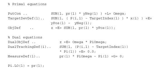

Note that constraints π l ≥ pl are defined using the lower bound attribute Pi.LO(l) = pr(l).
Of course, we know from linear programming theory (see Appendix PFO-A) that it is not necessary to write explicitly the dual problem. The optimal values of the dual variables are immediately at hand with the GAMS linear programming solver by using the attribute M for variables and equations. For instance, π l are the dual prices for (5.54), and πω is the dual price for (5.53). They are both displayed with: The reader can simply check that the values in TargetDevDef.M coincide with the Pi.L, and PutCon.M coincides with PiOmega.L, where Pi.L and PiOmega.L are the variables of the dual Model PFO-5.7.2.
In case the put/call model is unconstrained, the dual price PutCon.M is constant for different levels of the coefficient ω. By adding liquidity constraints - for example, by setting upper and lower bounds on the amounts held for each security - the dual price PutCon.M is a stepwise decreasing function of the coefficient ω, and the efficient frontier is a concave function of ω.
Model PFO-5.7.3 with liquidity constraints is reproduced here:


Model PFO-5.7.3 Put/call efficient portfolio with finite liquidity
(5.61)
(5.62)
(5.63)
(5.64)
(5.65)
(5.66)
We implement this model simply by setting the upper and lower bounds for each asset i ∈ U. We then collect the dual prices from TargetDevDef.M(l) and x.M(i). Note that the dual prices have to be taken with the opposite sign to correctly compute liquidity premium and discount.
We run Model PFO-5.7.3 with a mild and a tight set of liquidity constraints. These are given as: We show in Figure 5.8 the dual price πω for different risk levels ω. The model with mild liquidity constraints yields the curve with higher dual prices, and this is more pronounced when ω is small. In fact, to satisfy the put constraint when ω is small implies a strong trading (short or long) in the most attractive securities. When the model has tighter liquidity constraints, the gain in relaxing ω is less pronounced, since trading is already limited.

Liquidity constraints also have an influence on the put/call efficient frontiers. A tight bound on the trading activity will force the use of those securities that have the highest upside for a given downside. The trade-off rate between the call value and the put value is thus reduced, and the efficient frontier becomes more concave (see Figure 5.9).
Figure 5.8: Dual price πω for different risk levels ω. The two curves are drawn using two different sets of liquidity constraints. The model with less liquidity (tight constraints) yields lower dual prices as the trading activity is already bounded in a small range of values, and by relaxing ω the objective function improves only slightly.
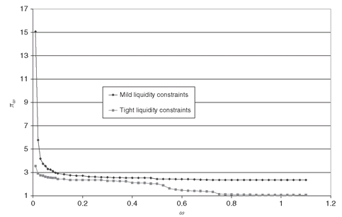
Figure 5.9: Put/call efficient frontiers using two different sets of liquidity constraints. The tighter the liquidity constraints, the more concave the efficient frontier, which is dominated by efficient frontiers with mild constraints on liquidity.
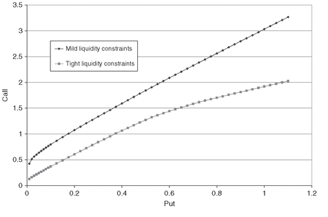
Figure 5.10: Liquidity premia and discounts for risk level ω = 0.475. Securities trading at their upper bounds yield a discount premium. By relaxing the upper bounds for such securities, the expected upside will increase; therefore, a discount is received to trade at the given bound.
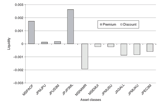
Finally, we determine the liquidity premia for a given risk level ω. As explained in Section PFO-5.7.1, the presence of upper and lower bounds on the amount held for each security generates liquidity cost. Model PFO-5.7.3 allows the estimate of such costs. In particular, if a security trades at the lower bound, the associated dual price will be greater than zero, and the liquidity premium is given by where,
 is the dual price linked with the lower bound constraint, and πl are the dual prices linked with the equation defining the deviations from the benchmark. Note that we did not explicitly write the bound constraints, since GAMS sets box constraints through the LO and UP variable attributes. We obtained the dual prices using the attribute M. The GAMS variable extension x.M(i) holds the dual prices
 which are negative for securities trading at their lower bound, and πi, which are positive for securities trading at their upper bound.
The GAMS code to compute the liquidity Premium(i) and Discount(i) is given below:


The term Price(i) carries the current asset prices (P0i ). Note that, from the properties of linear programming for dual variables, Premium(i) and Discount(i) can both be zero - if the security trades in between its bounds - but they cannot both be different than zero. Price(i) is thus given by the BenchMarkNeutralPrice(i) plus Premium(i) and minus Discount(i). Since we built the model such that the initial prices are all equal to one, we also expect that Price(i) is equal to one.
In Figure 5.10 we display the liquidity premium and discount for each asset. The security labeled MSPACF is traded at its lower bound; this means that we have to pay a premium to keep it in our portfolio. If no lower bound was set for MSPACF, the optimal solution will short as much as possible of this asset, thus improving the objective function. The opposite occurs for MSNAMR that is traded at its upper bound, and therefore yields a liquidity discount.
5.7.1 The FINLIB files
The GAMS source code and data for the models of this section are given in the following file:
• PutCall.gms
..................Content has been hidden....................
You can't read the all page of ebook, please click here login for view all page.
