Chapter 3
Mean-Variance Portfolio Optimization
3.1 Preview
In this chapter we develop the GAMS models for mean-variance portfolio optimization. The development is based on the discussion of Chapter PFO-3. The following models are discussed in this chapter and the GAMS source code for each is given in the associated FINLIB files:
Basics of mean-variance models are based on Section PFO-3.2. We set up the framework to trace mean-variance efficient frontiers. The relevant statistics - expected returns and variance-covariance matrixes - are estimated from historically observed data.
• MeanVar.gms
• Estimate.gms
Sharpe ratio model is based on Section PFO-3.2.2 with the optimal Sharpe ratio.
• Sharpe.gms
Portfolio limits are based on Section PFO-3.2.2. We determine portfolios with a limited number of assets, or minimum proportions, using binary variables.
• MeanVarShort.gms
• MeanVarMip.gms
• Borrow.gms
International mean-variance portfolio management formulates a large model for managing a portfolio of international stock and bond indices.
• InternationalMeanVar.gms
3.2 Basics of Mean-Variance Models
The classic mean-variance model addresses the question of trading off the portfolio expected return against its risk as measured by the variance of return. The model assumes normally distributed returns and multivariate normal correlation structures, but it is also applied in practice when the distributions are almost normal. For more details on the theoretical background of the model, see Section PFO-3.2.
Our first model is the basic mean-variance Model PFO-3.2.3, which we reproduce here:


Model PFO-3.2.3 Mean-variance efficient portfolios
(3.1)
(3.2)
(3.3)
We have available, in our data set, estimates of expected returns and the variance-covariance matrix for a universe of eight assets: an index of Italian government bonds with short maturity, some stock indices including the general Italian index, and a cash position in Euro as the risk-free asset. We compute the expected returns for each asset and the variance-covariance matrix through Estimate.gms (see Section 3.2.1 for details).
The output of Estimate.gms is dumped into a GDX container (Estimate.gdx), and the data needed are then loaded into MeanVar.gms by the GDX utility: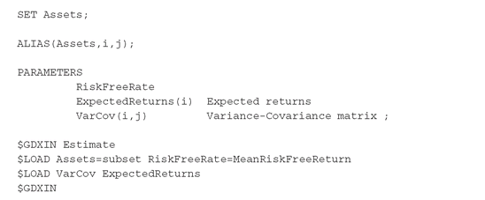

Note that the SET and PARAMETERS are first declared and then filled via the load call. In particular, the set Assets is assigned the parameter subset. The latter is defined and filled in Estimate.gms and dumped into the GDX container. VarCov is simply listed, without assignment, since this parameter has the same name as that contained in Estimate.gms.
In the VARIABLES section of the model we declare the vector of holdings of the assets. This vector is restricted to be positive since we are assuming for now that short sales are not allowed. In the model discussed in Section 3.2.2 we remove this restriction. Other variables are the expected return, the variance of the portfolio, and the objective function value.

The portfolio expected return (PortReturn) and the portfolio variance (PortVariance) are defined by the equations:
The variables x(i) measure the fraction of capital to be invested in each asset. By normalizing to one, the set of feasible portfolios - those whose weights add up to one - is identified by the following constraint: The objective value z is a weighted sum of the portfolio’s expected return, PortReturn, and its risk, PortVariance, where the parameter λ varies between zero and one.
The parameter lambda (λ in Model PFO-3.2.3) represents the investor risk attitude. If it is close to one, the investor is risk averse, emphasizing the risk component (variance) without regard to expected return. When it is zero the investor is risk-neutral.
Different risk attitudes are suitable for different investors. We therefore trace the mean-variance efficient frontier corresponding to portfolios that are optimal for different values of λ. In GAMS, this can be done using a FOR loop: This code segment will solve the model for values of λ ranging from zero to one in increments of 0.1.

The results of the optimization are stored in a file by means of the PUT statement. The data needed to plot the efficient frontier are the optimal portfolio variance (PortVariance.L) and the optimal portfolio return (PortReturn.L). With each mean-variance pair corresponding to a given value of λ, there is an optimal portfolio (x.L) stored in the same file.
An alternative way of writing and presenting the results obtained is through the GDX utility GDXXRW. In this case, data structures have to be declared in order to receive the output produced. As a starting point we define the set of points that will describe the efficient frontier.

To each point there will correspond a minimum variance, an expected return, and an optimal portfolio. Information about the solver status is also stored. All these parameters have to be indexed by p:

The optimization model is solved inside a LOOP statement indexed by p, and the results obtained are cast in the SummaryReport parameter.
The latter is “unloaded” into the GDX container Summary.gdx, and the GDX utility GDXXRW will produce the Excel file MeanVarianceFrontier.xls.

The values of the optimal (expected return, variance) pairs are shown in Figure 3.1. As expected, the portfolios corresponding to high risk aversion (large λ) have the lowest variances (around 0.01), but also the lowest expected returns (around 10%). In contrast, the portfolios for low risk-averse investors have variances greater than 0.5 and expected returns around 23%. In Figure 3.2 we show a set of portfolios for different values of λ. Note that the portfolios with the highest number of stocks correspond to the more risk-averse investors, as these investors diversify their portfolios to reduce their risk.
For λ = 0.1, only the assets EMERGT and NORD_AM (with the highest expected returns) are held, but as λ increases, the model diversifies into up to five assets, as risk is decreased together with the portfolio expected returns. It is typical behavior for the mean-variance model to diversify into a high number of assets when risk aversion is high. Such a portfolio can be impractical and costly to manage in practice, and in Section 3.4 we give an alternative model to address this problem.
An alternative formulation to Model PFO-3.2.3 minimizes the portfolio variance subject to the portfolio expected return reaching an investor-specified target μ (called mu in the GAMS formulation). We reproduce here Model PFO-3.2.2: 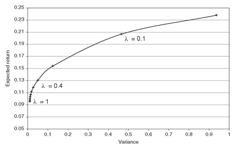
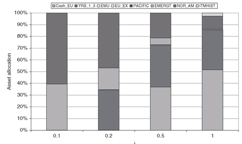
Figure 3.1: Mean-variance efficient frontier when short sales are not allowed. The parameter λ (lambda in the GAMS formulation) denotes the investor risk aversion. High values of λ (high risk aversion) are associated with low variances (low risk) and low returns. Low values of λ (low risk aversion) are associated with high variances (high risk) and high returns.

Figure 3.2: Composition of the optimal portfolios for varying values of λ (lambda in the GAMS model). As the risk aversion increases, the number of stocks in the portfolio increases as well. Investors with high risk aversion will pay in terms of reduction of their portfolio return to reduce risk.

Model PFO-3.2.2 Variance minimization
(3.4)
(3.5)
(3.6)
The two models are equivalent in the sense that they generate the same efficient frontier by varying lambda or mu, respectively. Of course, the latter model can be made infeasible by specifying a target return outside the range of expected returns given by the underlying asset universe. An example of this alternative formulation is found in Section 3.5.
3.2.1 Data estimation for the mean-variance model
The mean-variance model is usually based upon historical data, such as observed stock returns or stock index returns. We show here how this can be done based on monthly data over a 10-year time period for a large set of asset classes, including the eight classes used in the MeanVar.gms model. The complete data set is found in AssetsData.inc, and Estimate.gms estimates the data needed for mean-variance optimization using the time series of returns. This model extracts the expected returns and variances/covariances data used in the preceding section.
Let the observation times be denoted τt = (τ0 , τ, . . . , τT), where τ0 = January 1, 1990 and τT = January 1, 2000, and let Δ = be the time interval (one month) between observations. The observed prices are first converted to a common currency, the Italian Lira,1 and stored in the parameter data_ITL(t,i), for each time point t and asset i; the file ExchangeRates.inc contains exchange rates for each observation date.
We first calculate the annualized return of each stock in each period, Ret_ITL(t,i), using the continuous-time formula where Pti is the asset price called DATA_ITL(t,i) in the GAMS model, using the following statement:
(3.7)
The $-operator serves to exclude references to a non-existing observation prior to the first one available.
The discrete-time version of the formula for calculating returns, might be more familiar; either one could be used.
(3.8)
1 The data used predate the introduction of the Euro, on January 1, 2002, in most EU countries.
Given these returns, it is straightforward to calculate the expected returns over the entire observation period, and the covariances of returns among pairs of assets. Mean returns μi , and covariances of returns σij (see Equation PFO-2.1 and Definition PFO-2.3.6, respectively) are estimated as and
and Note that, unlike the definitions in PFO, we use the historical time periods to denote scenarios, adopting the simple bootstrapping method of Section PFO-9.4.1 for scenario generation, whereby it is assumed that every historical observation is a likely future scenario. The GAMS implementation is given by:
 where i1, i2 are aliases of the asset index i.
(3.9)

(3.10)


From the resulting data, MU and Q, we extract the input data for the MeanVar.gms model, ExpectedReturns and VarCov: where SUBSET is the subset of the assets we are interested in.

The whole input data set and the parameters computed are dumped into the GDX container Estimate.gdx. The latter can be used as input for other GAMS models (see previous section) and inspected, through the GAMSIDE application, to check consistency of the input data and results.
3.2.2 Allowing short sales
We now formulate the mean-variance model when short sales are allowed, i.e., when investors are allowed to sell securities they do not own. In GAMS, the short sales option can be modeled simply by removing the label POSITIVE from the declaration of the variables, x(i), and by allowing negative lower bounds on these variables in order to reflect any limits on short sales. A negative value for some variables in the optimal solution will indicate short sale of the corresponding asset.
The GAMS file MeanVarShort.gms solves the mean-variance model with two types of short sales restrictions: first, only a short position in each individual asset class of up to 20% of the total investment is allowed and second, the total short positions are limited to 50% of the total investments. These restrictions are implemented using negative lower bounds on asset positions in the first case, and accounting for short sales (through Short(i)) for each asset in the second case:
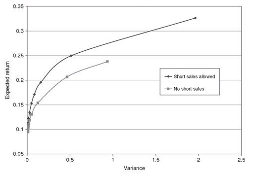


Figure 3.3: Mean-variance efficient frontiers with and without short sales; the frontier with short sales dominates; that is, for the same level of risk higher expected returns are attainable than without short sales.

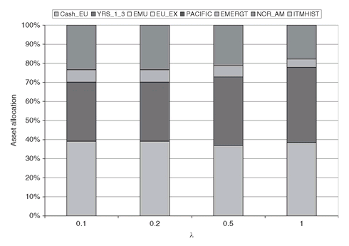
Figure 3.4: Portfolios for different levels of the risk aversion parameter (λ = 0.1, 0.2, 0.5, 1), when short sales are allowed.

As expected, the resulting portfolios have even better risk-reward characteristics. The resulting efficient frontier, together with the frontier obtained with no short sales, is shown in Figure 3.3. The optimal portfolios are now better diversified than the MeanVar model (see Figure 3.4), when also taking into account the short positions. Of course, when short sales are allowed, we also introduce the risk of getting caught in a “short squeeze.”
3.2.3 The FINLIB files
The GAMS source code and data for the models of this section are given in the following files:
• MeanVar.gms
• Estimate.gms
• MeanVarShort.gms
• Estimate.gdx
• AssetsUniverse.inc
• AssetsData.inc
• ExchangeRates.inc
3.3 Sharpe Ratio Model
The Sharpe model is closely related to the mean-variance model, but maximizes the Sharpe ratio (see Definition PFO-2.8.11), where
where =
= P -
P -  B is the excess return of the portfolio,
 P , over a benchmark portfolio return,
 B ;
B ; is the average excess return; and σd the standard deviation of excess returns of the portfolio P .
(3.11)
We use as a benchmark index the low-risk Euro Cash account, CASH_EU. The return and variance-covariance statistics are calculated as usual, but relative to the excess portfolio return over the benchmark.
The model in Estimate.gms performs these calculations: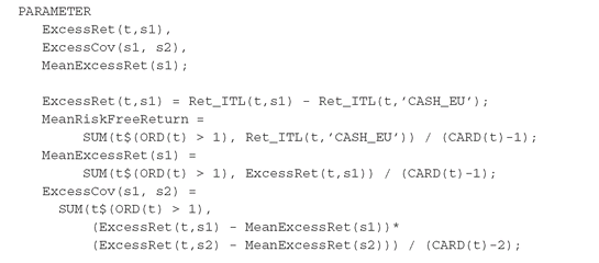

The excess returns are calculated with respect to the CASH_EU, which is assumed to be the risk-free asset. The model equations in Sharpe.gms follow directly:

Notice the need to put a strictly positive lower bound on the Variance variable because it is used as an argument of the square root function. In general, nonlinear solvers will not attempt to evaluate any nonlinear expressions until all linear constraints, including bounds, are satisfied.
The optimal Sharpe portfolio is similar to the optimal mean-variance portfolio obtained for λ = 0.2. It consists of about 35% Italian bonds of short maturity, about 20% emerging markets, and about 45% North American stocks. Recall from Theorem PFO-2.3.1 that this is the tangent portfolio.
Figure 3.5: Mean-variance efficient frontier when a risk-free asset is available.
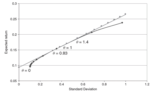
In Figure 3.5, we show how the efficient frontier changes once risk-free lending is allowed. The new linear efficient frontier dominates the previous one. The investor will split investments between the risk-free asset and the tangent portfolio fund, identified by θ = 1.
The scalar theta is obtained as the ratio between the volatility of the portfolio, and the volatility of the tangency portfolio,

A value of θ less than one implies that the investor is lending at the risk-free rate. Values of θ greater than one implies that investor is borrowing at the risk-free rate and investing the proceeds in the tangent portfolio.
3.3.1 Risk-free borrowing
The amount borrowed can be explicitly modeled in the mean-variance model. Following the extensions given in Section PFO-3.2.2, the relevant GAMS file implementing the model is given in Borrow.gms. We declare two variables, borrow_1 and borrow_2, to carry the amount of money borrowed at two different borrowing rates, BorrowRate_1 and BorrowRate_2. Given that BorrowRate_1 is less than BorrowRate_2, in order that the borrow_2 is different than zero, we must set an upper bound on the first variable, for example, borrow_1.UP = 2. Therefore, the investor will borrow at the BorrowRate_1 up to borrow_1.UP and the rest at the BorrowRate_2. The normalization constraint becomes: The normalization constraint shows that all the proceeds of the borrowing go into the portfolio; of course, the holdings will no longer sum up to one. The return of the portfolio is diminished by the amount of the borrowing times the relative rates; however, since the borrowing rates are risk-free the variance of the portfolio does not change.

For lambda = 0 only the return of the portfolio is relevant and, therefore, the model will try to maximize the expected return. This of course can be made as large as we like, as the amount of holdings increases by borrowing at the risk-free rate. Therefore, without a limit on the amount borrowed, the model instance with lambda = 0 is unbounded. This is shown in the output file where we report the status of the model after optimization. A value MODELSTAT = 3 means that the model is unbounded.
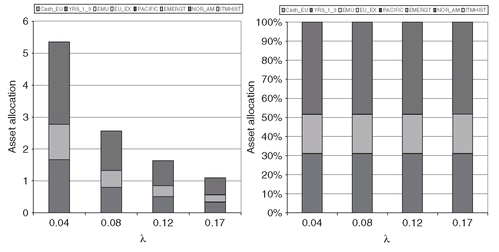
In Figure 3.6 (left), we show the absolute asset allocations for different values of lambda. Note that the lower the lambda (low risk aversion) the higher the amount borrowed and invested in the tangent portfolio. For example, when lambda = 0.04 the amount borrowed is 4.37, which means that more than four units of capital were borrowed and invested in the tangent portfolio in addition to one unit of own capital. To confirm that the proceeds of the borrowing are allocated in the tangent portfolio, we display in Figure 3.6 (right) the relative asset allocations obtained by normalizing the holdings with the available capital (one plus the borrowing). As expected, the portfolio compositions are the same for all values of the risk aversion parameter.
Figure 3.6: Absolute (left) and relative (right) asset allocations for different levels of the risk aversion parameter (λ = 0.04, 0.08, 0.12, 0.17), when borrowing at a risk-free rate is allowed. In this instance, none of the borrowing variables were bounded.
3.3.2 The FINLIB files
The GAMS source code and data for the models of this section are given in the following files:
• Sharpe.gms
• Borrow.gms
• Estimate.gdx
3.4 Diversification Limits and Transaction Costs
A general problem with the mean-variance model for risk-averse investors is that the optimal portfolios often consist of a large number of individual stock holdings, making them very expensive to manage. A natural question is how to limit the number of stocks held in the portfolio. There are two obvious ways to do so: either by explicitly modeling transaction costs and subtracting them from the expected returns, or by limiting the number of stocks held in the portfolio. Such requirements can be modeled quite simply, but the resulting models are nonlinear and contain discrete (binary) variables, and can be difficult to solve. The file MeanVarMip.gms contains a modification of the mean-variance model where the number of stocks in the portfolio is limited to StockMax: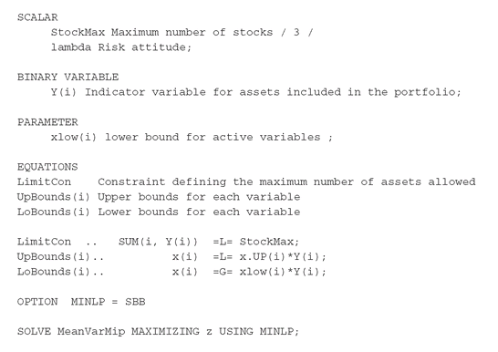

Figure 3.7: Mean-variance efficient frontiers with and without trading constraints.

This is a simple extension of the standard model given in MeanVar.gms, whereby binary variables Y(i) are used to count and limit the number of assets present in the portfolio. The constraints UpBounds(i) and LoBounds(i) force the variables included in the portfolio (i.e., those variables i for which Y(i) = 1) to stay between the upper and lower bound specified through the UP of the GAMS variables and the parameter xlow(i). Finally, the LimitCon constraint ensures that at most Stockmax different stocks enter the portfolio, i.e., at most Stockmax binary variables Y(i) can be 1. Note that if short sales are allowed, xlow(i) must be set to a negative value; the normalization constraint will ensure that there will be long positions to counterbalance the short ones.
This version of the mean-variance model (MeanVarMip.gms) is a mixed-integer, nonlinear program, MINLP. For high values of λ, where risk aversion causes diversification, the MeanVarMip model results in portfolios with only three assets. These portfolios are usually dominated by those obtained with the unconstrained MeanVar.gms (see Figure 3.7).
3.4.1 Transaction costs
Transaction costs can be easily introduced if such costs are proportional to transaction size. In such cases the return constraint is modified as follows (see also equation PFO-3.36): where PropCost is the proportional cost. A more realistic setting distinguishes a fixed cost FlatCost for transactions up to a certain amount, and a proportional cost thereafter. In this case the return constraint must include a binary variable to take into account the two cost regimes. To do so, we split the variables in two parts: x_0(i) accounts for amounts for which a fixed cost is paid, and x_1(i) accounts for amounts for which a proportional cost is paid. The total holdings are given by x(i) = x_0(i) + x_1(i).
We devote a part of the model in MeanVarMIP.gms to this case. The new equation definitions are: Note that equation ReturnDefWithCost, which defines the expected return of the portfolio, is made up of two components: one where the transaction fee is fixed, and a second where the transaction costs are proportional (see Equation PFO-3.38).

By setting the transaction costs to
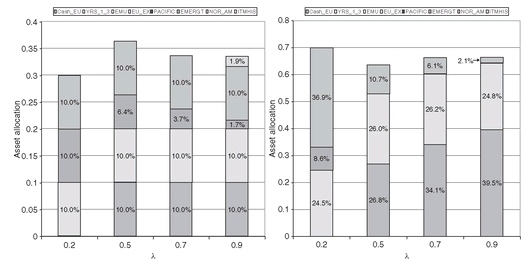 we obtain the portfolio displayed in Figure 3.8, for different values of λ. On the left, we report the asset allocations relative to x_0(i); on the right the asset allocations relative to x_1(i).

Figure 3.8: Asset allocations under fixed transaction costs (left), and asset allocations under proportional transaction costs (right), for different level of the risk aversion parameter (λ = 0.2, 0.5, 0.7, 0.9).

3.4.2 Portfolio revision
In this section we address the problem faced by portfolio managers when, for example, after a change in the parameters of the mean-variance model, they have to revise their portfolio. In such cases, however, one may wish to stay somewhat close to the existing portfolio. Hence a portfolio manager may set a target to stay within prespecified ranges of the current asset allocations.
In the third part of the model in MeanVarMIP.gms we implement zero-or-range constraints, which ensure that the asset allocation will either not change at all from its current value, or, if it does change, the changes will stay within a bounded range near the current allocation. Following the model given in Section PFO-3.2.4 we define the buying and selling variables by declaring: The new equations for portfolio revision are:
 Equation InventoryCon(i) defines, for each asset and for a given initial holding, the total holding, x(i), after selling and purchasing of assets. We split the range constraints in two inequalities, since GAMS does not deal explicitly with inequalities ranges; those are given by UpBuyLimits(i), UpSellLimits(i), LoBuyLimits(i) and LoSellLimits(i). The binary variables, Yb(i) and Ys(i), force the buy and sell variables to be zero or to stay within the prespecified range. Finally, the BuyTurnover constraint takes care of the total turnover. Note that, since the asset allocations must add up to one, the total turnover limits both the buy and the sell amounts.


In Figure 3.9 we show the asset allocation after the revision of the portfolio. The initial holdings are set equal to those of the optimal mean-variance portfolio with λ = 0.5 and no turnover constraints. By comparing Figure 3.9 with Figure 3.2, we note that the portfolio with λ = 0.5 did not change. As expected, when the expected returns and the variance-covariance matrix stay fixed or move little, the revision of the portfolio should have no effect. However, if we change the risk aversion parameter λ to 0.1 or 0.2, the new asset allocation will hit the bounds of the selling and purchasing variables.
Figure 3.9: Asset allocation after portfolio revision. The initial holding is set to the unconstrainedoptimal portfolio with λ = 0.5.
3.4.3 The FINLIB files
The GAMS source code and data for the models of this section are given in the following files:
• MeanVarMip.gms
• Estimate.gdx
3.5 International Portfolio Management
In this section we build large-scale mean-variance models for managing international portfolios of bond and stock indices. The models are based on the entire raw data set contained in AssetsData.inc and ExchangeRates.inc. As seen in Section 3.2, the data required by the models are computed by Estimate.gms, and filled in the proper sets and parameters directly from the GDX container Estimate.gdx:

The raw data consists of monthly observations over a 10-year period (January 1, 1990 through January 1, 2000) of prices of 46 different asset classes, including a risk-free asset. These are 23 Italian sector stock indices and the general Italian stock index, three Italian bond indices, seven international bond indices, five international stock indices, three international cash rates and three US corporate bond sector indices. The risk-free asset is an Italian cash account. The data file also contains a time series of exchange rates between all relevant currencies and the Italian Lira, which is used as the common numeraire.
This model deals with asset allocation among broad asset classes by an Italian investor. Our investor first has to determine the structure of her portfolio by allocating funds in the major stock indices of the Milano stock exchange, and government bonds of different maturities. She then extends the allocation to international asset classes, namely government bonds, and finally invests in addition in US corporate bonds. We will see how the efficient frontier can be pushed out when diversifying internationally. However, we must note that all returns are measured in the foreign currency (e.g., in USD for the corporate bond market) so that foreign exchange risk is not included in this model. We can either assume that our Italian investor hedges currency exposure with forward contracts, or we can be patient until Section 7.2.3 to incorporate hedging decisions in asset allocation models.
The portfolio selection in InternationalMeanVar.gms is structured as follows:
Step 1. Include only Italian stock indices; this model contains 23 assets.
Step 2. Augment the assets universe to include bond indices of the Italian market; this model contains 26 assets.
Step 3. Add international stock indices. In particular we added five asset classes representing the major international stock markets, bringing the total number of assets to 31.
Step 4. Incorporate all asset classes, which include six international government bond indices and three corporate bond indices, for a total of 40 asset classes.
Step 5. Include a risk free asset, in addition to all risky assets above.
Step 6. Finally, the Italian general stock index It_general, is treated as a target liability. The Italian assets (23 stock indices) are then used to construct a mean-variance portfolio that is highly correlated with the target liability, and thus it tracks (or synthesizes) the liability.
We trace now the efficient frontiers for each step of our models. In the MeanVar.gms model this was done by changing the weight, lambda, between the portfolio expected return and its variance, but in the InternationalMeanVar.gms model we use the variance minimization Model PFO-3.2.2, and set a target return, MU_TARGET, which varies from zero to the largest expected return among the assets, MAX_MU.
3.5.1 Implementation with dynamic sets
In this section we describe the model in InternationalMeanVar.gms and its included data files.
The asset universe set and a number of subsets, corresponding to the different asset subsets used in the models, are declared in the include file AssetUniverse.inc. For example, the subset IT_ALL is given by:  The subsets allow us to change dynamically and in a flexible way the universe of assets that participate in each of the six models. This is done through a dynamic set, ACTIVE, which at any point contains the set of active assets:
 Of course, the basic decision variables and constraints are unchanged from the previous models:
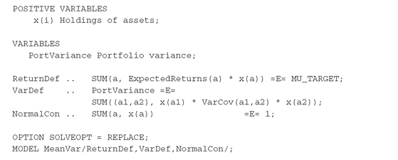 Notice that all indexing in the constraints is done using the indices a, a1, and a2, which are aliases of the set ACTIVE. This set will be initialized to different values for the models in Steps 1 to 5. When it is re-initialized, the aliases a, a1, and a2 change their domains as well.


By dynamically changing the contents of ACTIVE, we are effectively changing the domain of the constraint summations. Hence, before solving each of the five models, the following is executed:
Step 1. Italian stocks
Step 2. Italian stocks and bonds
Step 3. Italian and international stock indices
Step 4. All indices
Step 5. All Italian stock indices plus risk-free rate. In this case the data set is the same as Step 4.
Step 6. Include the general index as liability.
The action for Step 2, for instance, assigns to the active set the assets contained in the IT_ALL subset.
The decision variables x(i) are defined over the whole asset universe, but in any specific model only a subset is used. The default in GAMS is to leave the values of x(i) from the previous steps unchanged as it proceeds to solve the next step. This is unfortunate for our purposes, since when we display the vector of optimal investments, it may appear, for instance, that corporate bonds are part of the universe when our model does not include them since the corresponding x(i) may have a non-zero value from the solution of the previous step.
The GAMS option changes this behavior so that variables that do not participate in a specific model have their values reset to 0 so that they do not show up in the solution again.
Finally, in Step 6, we include a liability and essentially use the Italian assets to track the Italian general stock index. This model is very similar in essence to the Sharpe model of Section 3.3, but instead of calculating the excess returns and variance-covariances relative to the general stock index, we now use a different approach: the general stock index is included in the portfolio, but with a fixed “proportion” of -1, indicating that it is now really a liability (or a short position). The remaining part of the model is unchanged, except that the sum of asset proportions - including the liability position -1 - now must sum to 0: In this model, with its relatively large set of assets, the optimal portfolios often contain assets with very small proportions, even less than 1%. This indicates that the model would be a good candidate, in a real-world setting, for the zero-or-range constraints presented in Section 3.4. See also Section 5.3.1 and Section PFO-5.3.3 for an alternative formulation of this problem using scenarios.

Figure 3.10: Mean-variance frontiers when using increasingly larger sets of assets.
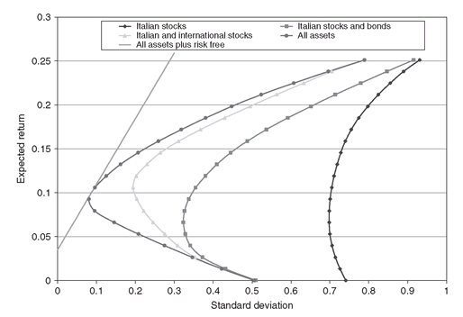
In Figure 3.10 we display the mean-variance frontier for each set of assets. Since each set includes the previous one, the mean-variance frontier dominates the ones obtained by optimizing over a smaller asset set.
3.5.2 The FINLIB files
The GAMS source code and data for the models of this section are given in the following files:
• InternationalMeanVar.gms
• Estimate.gdx
..................Content has been hidden....................
You can't read the all page of ebook, please click here login for view all page.
