CHAPTER 2
Fundamentals of Digital Audio

The digital techniques used to record, reproduce, store, process, and transmit digital audio signals entail concepts foreign to analog audio methods. In fact, the inner workings of digital audio systems bear little resemblance to analog systems. Because audio itself is analog in nature, digital systems employ sampling and quantization, the twin pillars of audio digitization, to represent the audio information. Any sampling system is bound by the sampling theorem, which defines the relationship between the message and the sampling frequency. In particular, the theorem dictates that the message be bandlimited. Precaution must be taken to prevent a condition of erroneous sampling known as aliasing. Quantization error occurs when the amplitude of an analog waveform is represented by a binary word; effects of the error can be minimized by dithering the audio waveform prior to quantization.

Discrete Time Sampling

With analog recording, a tape is continuously modulated or a groove is continuously cut. With digital recording, discrete numbers must be used. To create these numbers, audio digitization systems use time sampling and amplitude quantization to encode the infinitely variable analog waveform as amplitude values in time. Both of these techniques are considered in this chapter. First, let’s consider discrete time sampling, the essence of all digital audio systems.

Time seems to flow continuously. The hands of an analog clock sweep across the clock face covering all time as it passes by. A digital readout clock also tells time, but with a discretely valued display. In other words, it displays sampled time. Similarly, music varies continuously in time and can be recorded and reproduced either continuously or discretely. Discrete time sampling is the essential mechanism that defines a digital audio system, permits its analog-to-digital (A/D) conversion, and differentiates it from an analog system.

However, a nagging question immediately presents itself. If a digital system samples an audio signal discretely, defining the audio signal at distinct times, what happens between samples? Haven’t we lost the information present between sample times? The answer, intuitively surprising, is no. Given correct conditions, no information is lost due to sampling between the input and output of a digitization system. The samples contain the same information as the conditioned unsampled signal. To illustrate this, let’s try a conceptual experiment.

Suppose we attach a movie camera to the handlebars of a BMW motorcycle, go for a ride, and then return home and process the film. Auditioning this piece of avant-garde cinema, we discover that the discrete frames of film reproduce our ride. But when we traverse bumpy pavement, the picture is blurred. We determine that the quick movements were too fast for each frame to capture the change. We draw the following conclusion: if we increased the frame rate, using more frames per second, we could capture quicker changes. Or, if we complained to city hall and the bumpy pavement was smoothed, there would be no blur even at slower frame rates. We settle on a compromise—we make the roads reasonably smooth, and then we use a frame rate adjusted for a clean picture.

The analogy is somewhat clumsy. (For starters, cinema comprises a series of discontinuous still images—it is the brain itself that creates the illusion of a continuum. An audio waveform played back from a digital source really is continuous because of the interpolation function used to create it.) Nevertheless, the analogy shows that the discrete frames of a movie create a moving picture, and similarly the samples of a digital audio recording create a continuous signal. As noted, sampling is a lossless process if the input signal is properly conditioned. Thus, in a digital audio system, we must smooth out the bumps in the incoming signal. Specifically, the signal is lowpass filtered; that is, the frequencies that are too high to be properly sampled are removed. We observe that a signal with a finite frequency response can be sampled without loss of information; the samples contain all the information contained in the original signal. The original signal can be completely recovered from the samples. Generally, we observe that there exists a method for reconstructing a signal from its amplitude values taken at periodic points in time.

The Sampling Theorem

The idea of sampling occurs in many disciplines, and the origin of sampling theorems comes from many sources. Most audio engineers recognize American engineer Harry Nyquist as the author of the sampling theorem that founded the discipline of modern digital audio. The recognition is well-founded because it was Nyquist who expressed the theorem in terms that are familiar to communications engineers. Nyquist, who was born in Sweden in 1889, and died in Texas in 1976, worked for Bell Laboratories and authored 138 U.S. patents. However, the story of sampling theorems predates Nyquist.

When he was not busy designing military fortifications for Napoleon, French mathematician Augustin-Louis Cauchy contemplated statistical sampling. In 1841, he showed that functions could be nonuniformly sampled and averaged over a long period of time. At the turn of the century, it was thought (incorrectly) that a function could be successfully sampled at a frequency equal to the highest frequency. In 1915, Scottish mathematician E. T. Whittaker, working with interpolation series, devised perhaps the first mathematical proof of a general sampling theorem, showing that a band-limited function can be completely reconstructed from samples. In 1920, Japanese mathematician K. Ogura similarly proved that if a function is sampled at a frequency at least twice the highest function frequency, the samples contain all the information in the function, and can reconstruct the function. Also in 1920, American engineer John Carson devised an unpublished proof that related the same result to communications applications.

It was Nyquist who first clarified the application of sampling to communications, and published his work. In 1925, in a paper titled “Certain Factors Affecting Telegraph Speed,” he proved that the number of telegraph pulses that can be transmitted over a telegraph line per unit time is proportional to the bandwidth of the line. In 1928, in a paper titled “Certain Topics in Telegraph Transmission Theory,” he proved that for complete signal reconstruction, the required frequency bandwidth is proportional to the signaling speed, and that the minimum bandwidth is equal to half the number of code elements per second. Subsequently, Russian engineer V. A. Kotelnikov published a proof of the sampling theorem in 1933.

American mathematician Claude Shannon unified and proved many aspects of sampling, and also founded the larger science of information theory in his 1948 book, A Mathematical Theory of Communication. Shannon’s 1937 master’s thesis, “A Symbolic Analysis of Relay and Switching Circuits,” showed that circuits could use Boolean algebra to solve logical or numerical problems; his work was called “possibly the most important, and also the most famous, master’s thesis of the century.” Shannon, a distant relative of Thomas Edison, could also juggle three balls while riding a unicycle. Today, engineers usually attribute the sampling theorem to Shannon or Nyquist. The half-sampling frequency is usually known as the Nyquist frequency.

Whoever gets the credit, the sampling theorem states that a continuous bandlimited signal can be replaced by a discrete sequence of samples without loss of any information and describes how the original continuous signal can be reconstructed from the samples; furthermore, the theorem specifies that the sampling frequency must be at least twice the highest signal frequency. More specifically, audio signals containing frequencies between 0 and S/2 Hz can be exactly represented by S samples per second. Moreover, in general, the sampling frequency must be at least twice the bandwidth of a sampled signal. When the lowest frequency of the bandwidth of interest is zero, then the signal’s bandwidth equals the highest frequency. The sampling theorem is applied widely and diversely throughout engineering, science, and mathematics.

Nyquist Frequency

When the sampling theorem is applied to audio signals, the input audio signal is low-pass filtered, so that it is bandlimited with a frequency response that does not exceed the Nyquist (S/2) frequency. Ideally, the lowpass filter is designed so that the only signals removed are those high frequencies that lie above the high-frequency limit of human hearing. The signal can now be sampled to define instantaneous amplitude values. The sampled bandlimited signal contains the same information as the unsampled bandlimited signal. At the system output, the signal is reconstructed, and there is no loss of information (due to sampling) between the output signal and the input filtered signal. From a sampling standpoint, the output signal is not an approximation; it is exact. The bandlimited signal is thus re-created, as shown in Fig. 2.1.

Consider a continuously changing analog function that has been sampled to create a series of pulses. The amplitude of each pulse, determined through quantization, yields a number that represents the signal amplitude at that instant. To quantify the situation, we define the sampling frequency as the number of samples per second. Its reciprocal, sampling rate, defines the time between each sample. For example, a sampling frequency of 48,000 samples per second corresponds to a rate of 1/48,000 seconds. A quickly changing waveform—that is, one with high frequencies—requires a higher sampling frequency. Thus, the digitization system’s sampling frequency determines the high frequency limit of the system. The choice of sampling frequency is thus one of the most important design criteria of a digitization system, because it determines the audio bandwidth of the system.

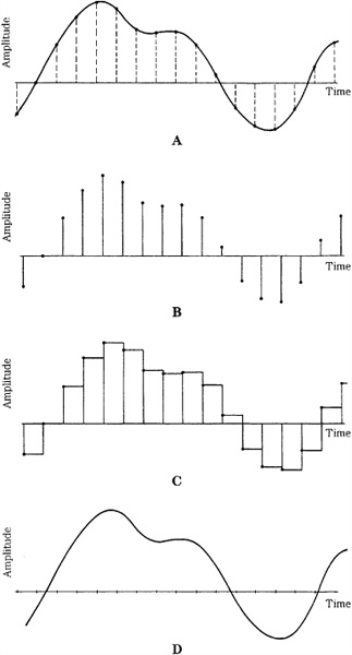
FIGURE 2.1 With discrete time sampling, a bandlimited signal can be sampled and reconstructed without loss because of sampling. A. The input analog signal is sampled. B. The numerical values of these samples are stored or transmitted (effect of quantization not shown). C. Samples are held to form a staircase representation of the signal. D. An output lowpass filter interpolates the staircase to reconstruct the input waveform.

The sampling theorem precisely dictates how often a waveform must be sampled to provide a given bandwidth. Specifically, as noted, a sampling frequency of S samples per second is needed to completely represent a signal with a bandwidth of S/2 Hz. In other words, the sampling frequency must be at least twice the highest audio frequency to achieve lossless sampling. For example, an audio signal with a frequency response of 0 to 24 kHz would theoretically require a sampling frequency of 48 kHz for proper sampling. Of course, a system could use any sampling frequency as needed. It is crucial to observe the sampling theorem’s criteria for limiting the input signal to no more than half the sampling frequency (the Nyquist frequency). An audio frequency above this would cause aliasing distortion, as described later in this chapter. A lowpass filter must be used to remove frequencies above the half-sampling frequency limit. A lowpass filter is also placed at the output of a digital audio system to remove high frequencies that are created internally in the system. This output filter reconstructs the original waveform. Reconstruction is discussed in more detail in Chap. 4.

Another question presents itself with respect to the sampling theorem. We observe that when low audio frequencies are sampled, because of their long wavelengths, many samples are available to represent each period. But as the audio frequency increases, the periods are shorter and there are fewer samples per period. Finally, in the theoretical limiting case of critical sampling, at an audio frequency of half the sampling frequency, there are only two samples per period. However, even two samples can represent a waveform. For example, consider the case of a 48-kHz sampling frequency and an audio input of 24-kHz sine wave. The sampler produces two samples, which will yield a 24-kHz square wave. In itself, this waveform is quite unlike the original sine wave. However, a lowpass filter at the output of the digital audio system removes all frequencies higher than the half-sampling frequency. (The 24-kHz square wave consists of odd harmonics—sine waves starting at 24 kHz.) With all higher frequency content removed, the output of the system is a reconstructed 24-kHz sine wave, the same as the sampled waveform. We know that the sampled waveform was a sine wave because the input lowpass filter will not pass higher waveform frequencies to the sampler. Similarly, a digitization system can reproduce all information from 0 to S/2 Hz, including sine wave reproduction at S/2 Hz; even in the limiting case, the sampling theorem is valid. Conversely, all information above S/2 is removed from the signal. We can state that higher sampling frequencies permit recording and reproduction of higher audio frequencies. But given the design criteria of an audio frequency bandwidth, higher sampling frequencies will not improve the fidelity of those signals already within the bandlimited frequency range.

For critical sampling, there is no guarantee that the sample times will coincide with the maxima and minima of the waveform. Sample times could coincide with lower-amplitude parts of the waveform, or even coincide with the zero-axis crossings of the waveform. In practice, this does not pose a problem. Critical sampling is not attempted; a sampling margin is always present. As we have seen, to satisfy the sampling theorem, a lowpass filter must precede the sampler. Lowpass filters cannot attenuate the signal precisely at the Nyquist frequency so a guard band is employed. The filter’s cutoff frequency characteristic starts at a lower frequency, for example, at 20 kHz, allowing several thousand Hertz for the filter to attenuate the signal sufficiently. This ensures that no frequency above the Nyquist frequency enters the sampler. The waveform is typically not critically sampled; there are always more than two samples per period. Furthermore, the phase relationship between samples and waveforms is never exact because acoustic waveforms do not synchronize with a sampler. Finally, when we examine the sampling theorem more rigorously in Chap. 4, we will see that parts of the waveform lying between samples can be captured and reproduced by sampling. We shall see that the output signal is not reconstructed sample by sample; rather, it is formed from the summation of the response of many samples. It is also worth noting that the bandwidth of any practical analog audio signal is also limited. No analog audio system has infinite bandwidth. The finite bandwidth of audio signals shows that the continuous waveform of an analog signal or the samples of a digital signal can represent the same information.

The need to bandlimit the audio signal is not as detrimental as it might first appear. The upper frequency limit of the audio signal can be extended as far as needed, so long as the appropriate sampling frequency is employed. For example, depending on the application, sampling frequencies from 8 kHz to 192 kHz may be used. The trade-off, of course, is the demand placed on the speed of digital circuitry and the capacity of the storage or transmission medium. Higher sampling frequencies require that circuitry operate faster and that larger amounts of data be conveyed. Both are ultimately questions of economics. Manufacturers selected a sampling frequency of 44.1 kHz for the Compact Disc, for example, because of its size, playing time, and cost of the medium. On the other hand, DVD-Audio and Blu-ray discs can employ sampling frequencies up to 192 kHz.

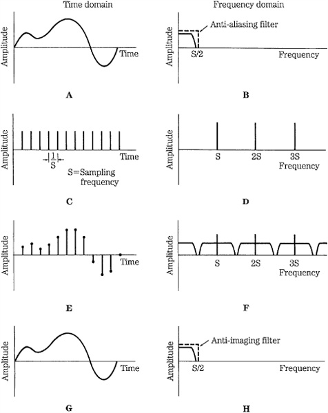
FIGURE 2.2 Time domain (left column) and frequency domain (right column) signals illustrate the process of bandlimited waveform sampling and reconstruction. A. Input signal after anti-aliasing filter. B. Spectrum of input signal. C. Sampling signal. D. Spectrum of the sampling signal. E. Sampled input signal. F. Spectrum of the sampled input signal. G. Output signal after anti-imaging filter. H. Spectrum of the output signal.

The entire sampling (and desampling) process is summarized in Fig. 2.2. The signals involved in sampling are shown at different points in the processing chain. Moreover, the left half of the figure shows the signals in the time domain and the right half portrays the same signals in the frequency domain. In other words, we can observe a signal’s amplitude over time, as well as its frequency response. We observe in Figs. 2.2A and B that the input audio signal must be bandlimited to the half-sampling frequency S/2, using a lowpass anti-aliasing filter. This filter removes all components above the Nyquist frequency of S/2. The sampling signal in Figs. 2.2C and D recurs at the sampling frequency S, and its spectrum consists of pulses at multiples of the sampling frequency: S, 2S, 3S, and so on. When the audio signal is sampled, as shown in Figs. 2.2E and F, the signal amplitude at sample times is preserved; however, this sampled signal contains images of the original spectrum centered at multiples of the sampling frequency. To reproduce the sampled signal, as in Figs. 2.2G and H, the samples are passed through a lowpass anti-imaging filter to remove all images above the S/2 frequency. This filter interpolates between the samples of the waveform, recreating the input, bandlimited audio signal. As described in Chap. 4, the output filter’s impulse response uniquely reconstructs the sample pulses as a continuous waveform.

The sampling theorem is unequivocal: a bandlimited signal can be sampled; stored, transmitted, or processed as discrete values; desampled; and reconstructed. No band-limited information is lost through sampling. The reconstructed waveform is identical to the bandlimited input waveform. Sampling theorems such as the Nyquist theorem prove this conclusively. Of course, after it has time-sampled the signal, a digital system also must determine the numerical values it will use to represent the waveform amplitude at each sample time. This question of quantization is explained subsequently in this chapter. For a more detailed discussion of discrete time sampling, and a concise mathematical demonstration of the sampling theorem, refer to the Appendix.

Aliasing

Aliasing is a kind of sampling confusion that can originate in the recording side of the signal chain. Just as people can take different names and thus confuse their identity, aliasing can create false signal components. These erroneous signals can appear within the audio bandwidth and are impossible to distinguish from legitimate signals. Obviously, it is the designer’s obligation to prevent such distortion from ever occurring. In practice, aliasing is not a serious limitation. It merely underscores the importance of observing the criteria of the sampling theorem.

We have observed that sampling is a lossless process under certain conditions. Most important, the input signal must be bandlimited with a lowpass filter. If this is not done, the signal might be undersampled. Consider another conceptual experiment: use your motion picture camera to film me while I drive away on my motorcycle. In the film, as I accelerate, the spokes of the wheels rotate forward, appear to slow and stop, then begin to rotate backward, rotate faster, then slow and stop, and appear to rotate forward again. This action is an example of aliasing. The motion picture camera, with a frame rate of 24 frames per second, cannot capture the rapid movement of the wheel spokes.

Aliasing is a consequence of violating the sampling theorem. The highest audio frequency in a sampling system must be equal to or less than the Nyquist frequency. If the audio frequency is greater than the Nyquist frequency, aliasing will occur. As the audio frequency increases, the number of sample points per period decreases. When the Nyquist frequency is reached, there are two samples per period, the minimum needed to record the audio waveform. With higher audio frequencies, the sampler will continue to produce samples at its fixed rate, but the samples create false information in the form of alias frequencies. As the audio frequency increases, a descending alias frequency is created. Specifically, if S is the sampling frequency, F is a frequency higher than the half-sampling frequency, and N is an integer, then new frequencies F_f are created at F_f = ± NS ± F. In other words, alias frequencies appear back in the audio band (and the images of the audio band), folded over from the sampling frequency. In fact, aliasing is sometimes called foldover. Although disturbing, this is not totally surprising. Sampling is a kind of modulation; in fact, sampling is akin to the operation of a hetero-dyne demodulator in an amplitude modulation (AM) radio. A local oscillator multiplies the input signal to move its frequency down to the standard intermediate frequency (IF). Although the effect is desirable in radios, aliasing in digital audio systems is undesirable.

Consider a digitization system sampling at 48 kHz. Further, suppose that a signal with a frequency of 40 kHz has entered the sampler, as shown in Fig. 2.3. The primary alias component results from S − F = F_f or 48 − 40 = 8 kHz. The sampler produces the improper samples, faithfully recording a series of amplitude values at sample times. Given those samples, the device cannot determine which was the intended frequency: 40 kHz or 8 kHz. Furthermore, recall that a lowpass filter at the output of a digitization system smoothes the staircase function to reconstruct the original signal. The output filter removes content above the Nyquist frequency. In this case, following the output filter, the 40-kHz signal would be removed, but the 8-kHz alias signal would remain, containing samples as innocuous as a legitimate 8-kHz signal. That unwanted signal is a distortion in the audio signal.

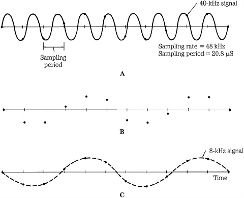
FIGURE 2.3 An input signal greater than the half-sampling frequency will generate an alias signal, at a lower frequency. A. A 40-kHz signal is sampled at 48 kHz. B. Samples are saved. C. Upon reconstruction, the 40-kHz signal is filtered out, leaving an aliased 8-kHz signal.

There are other manifestations of aliasing. Although only the S − F component appears as an interfering frequency in the audio band, an alias component will appear in the audio band, no matter how high in frequency F becomes. Consider a sampling frequency of 48 kHz; a sweeping input frequency from 0 to 24 kHz would sound fine, but as the frequency sweeps from 24 kHz to 48 kHz, it returns as a frequency descending from 24 kHz to 0. If the input frequency sweeps from 48 kHz to 72 kHz, it appears again from 0 to 24 kHz, and so on.

Alias components occur not only around the sampling frequency, but also in the multiple images produced by sampling (see Fig. 2.2F). When the sampling theorem is obeyed, the audio band and image bands are separate, as shown in Figs. 2.4A and B. However, when the audio band extends past the Nyquist frequency, the image bands overlap, resulting in aliasing as shown in Figs. 2.4C and D. All these components would be produced in an aliasing scenario: ± S ± F, ± 2S ± F, ± 3S ± F, and so on. For example, given a 48-kHz sampler and a 29-kHz input signal, some of the resulting alias frequencies would be 19, 67, 77, 115, 125, 163, and 173 kHz, as shown in Fig. 2.4D. With a sine wave, aliasing is limited to the one and only partial of a sine wave. With complex tones, content is generated for all spectra above the Nyquist frequency.

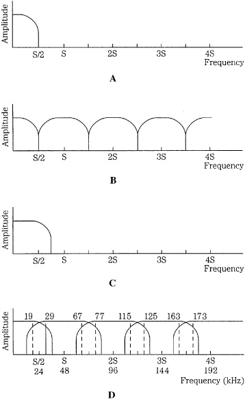
FIGURE 2.4 Spectral views of correct sampling and incorrect sampling causing aliasing. A. An input signal bandlimited to the Nyquist frequency. B. Upon reconstruction, images are contained within multiples of the Nyquist frequency. C. An input signal that is not bandlimited to the Nyquist frequency. D. Upon reconstruction, images are not contained within multiples of the Nyquist frequency; this spectral overlap is aliasing; for example, a 29-kHz signal will alias in a 48-kHz sampler.

In practice, aliasing can be overcome. In fact, in a properly designed digital recording system, aliasing does not occur. The solution is straightforward: the input signal is bandlimited with a lowpass (anti-aliasing filter) that provides significant attenuation at the Nyquist frequency to ensure that the spectral content of the sampled signal never exceeds the Nyquist frequency. An ideal anti-aliasing filter would have a “brick-wall” characteristic with instantaneous and infinite attenuation in the stopband. Practical anti-aliasing filters have a transition band above the Nyquist frequency, and attenuate stopband frequencies to below the resolution of the A/D converter. In practice, as described in Chap. 3, most systems use an oversampling A/D converter with a mild lowpass filter, high initial sampling frequency, and decimation processing to prevent aliasing at the downsampled output sampling frequency. This ensures that the system meets the demands of the sampling theorem; thus, aliasing cannot occur.

It is critical to observe the sampling theorem, and lowpass filter the input signal in a digitization system. If aliasing is allowed to occur, there is no technique that can remove the aliased frequencies from the original audio bandwidth.

Quantization

A measurement of a varying event is meaningful if both the time and the value of the measurement are stored. Sampling represents the time of the measurement, and quantization represents the value of the measurement, or in the case of audio, the amplitude of the waveform at sample time. Sampling and quantization are thus the fundamental components of audio digitization, and together can characterize an acoustic event. Sampling and quantization are variables that determine, respectively, the bandwidth and resolution of the characterization. An analog waveform can be represented by a series of sample pulses; the amplitude of each pulse yields a number that represents the analog value at that instant. With quantization, as with any analog measurement, accuracy is limited by the system’s resolution. Because of finite word length, a quantizer’s resolution is limited, and a measuring error is introduced. This error is akin to the noise floor in an analog audio system; however, perceptually, it can be more intrusive because its character can vary with signal amplitude.

With uniform quantization, an analog signal’s amplitude at sample times is mapped across a finite number of quanta of equal size. The infinite number of amplitude points on the analog waveform must be quantized by the finite number of quanta levels; this introduces an error. A high-quality representation requires a large number of levels; a high-quality music signal might require, for example, 65,536 amplitude levels or more. However, a few pulse-code modulation (PCM) levels can still carry information content; for example, just two amplitude levels can (barely) convey intelligible speech.

Consider two voltmeters, one analog and one digital, each measuring the voltage corresponding to an input signal. Given a good meter face and a sharp eye, we might read the analog needle at 1.27 V (volts). A digital meter with only two digits might read 1.3 V. A three-digit meter might read 1.27 V, and a four-digit meter might read 1.274 V. Both the analog and digital measurements contain errors. The error in the analog meter is caused by the ballistics of the mechanism and the difficulty in reading the meter. Even under ideal conditions, the resolution of any analog measurement is limited by the measuring device’s own noise.

With the digital meter, the nature of the error is different. Accuracy is limited by the resolution of the meter—that is, by the number of digits displayed. The more digits, the greater the accuracy, but the last digit will round off relative to the actual value; for example, 1.27 V would be rounded to 1.3 V. In the best case, the last digit would be completely accurate; for example, a voltage of exactly 1.3000 V would be shown as 1.3 V. In the worst case, the rounded off digit will be one-half interval away; for example, 1.250 V would be rounded to 1.2 V or 1.3 V. Similarly, if a binary system is used for the measurement, we say that the error resolution of the system is one-half of the least significant bit (LSB). For both analog and digital systems, the problem of measuring an analog phenomenon such as amplitude leads to error. As far as voltmeters are concerned, a digital readout is an inherently more robust measurement. We gain more concise information about an analog event when it is characterized in terms of digital data. Today, an analog voltmeter is about as common as a slide rule.

Quantization is thus the technique of measuring an analog audio event to form a numerical value. A digital system uses a binary number system. The number of possible values is determined by the length of the binary data word—that is, the number of bits available to form the representation. Just as the number of digits in a digital voltmeter determines resolution, the number of bits in a digital audio recorder also determines resolution. Clearly, the number of bits in the quantizing word is an arbitrary gauge of accuracy; other limitations may exist. In practice, resolution is primarily influenced by the quality of the A/D converter.

Sampling of a bandlimited signal is theoretically a lossless process, but choosing the amplitude value at the sample time certainly is not. No matter what the choice of scales or codes, digitization can never perfectly encode a continuous analog function. An analog waveform has an infinite number of amplitude values, but a quantizer has a finite number of intervals. The analog values between two intervals can only be represented by the single number assigned to that interval. Thus, the quantized value is only an approximation of the actual.

Signal-to-Error Ratio

With a binary number system, the word length determines the number of quantizing intervals available; this can be computed by raising the word length to the power of 2. In other words, an n-bit word would yield 2ⁿ quantization levels. The number of levels determined by the first n = 1 to 24 bits are listed in Table 2.1. For example, an 8-bit word provides 2⁸ = 256 intervals and a 16-bit word provides 2¹⁶ = 65,536 intervals. Note that each time a bit is added to the word length, the number of levels doubles. The more bits, the better the approximation; but as noted, there is always an error associated with quantization because the finite number of amplitude levels coded in the binary word can never completely accommodate an infinite number of analog amplitudes.

It is difficult to appreciate the accuracy achieved by a 16-bit measurement. An analogy might help: if sheets of typing paper were stacked to a height of 22 feet, a single sheet of paper would represent one quantization level in a 16-bit system. Longer word lengths are even more impressive. In a 20-bit system, the stack would reach 352 feet. In a 24-bit system, the stack would tower 5632 feet in height—over a mile high. The quantizer could measure that mile to an accuracy equaling the thickness of a piece of paper. If a single page were removed, the least significant bit would change from 1 to 0. Looked at in another way, if the driving distance between the Empire State Building and Disneyland was measured with 24-bit accuracy, the measurement would be accurate to within 11 inches. A high-quality digital audio system thus requires components with similar tolerances—not a trivial feat.

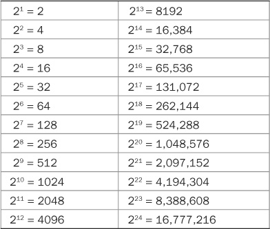
TABLE 2.1 The number (N) of quantization intervals in a binary word is N = 2ⁿ, where n is the number of bits in the word.

At some point, the quantizing error approaches inaudibility. Most manufacturers have agreed that 16 to 20 bits provide an adequate representation; however, that does not rule out longer data words or the use of other signal processing to optimize quantization and thus reduce quantization error level. For example, the DVD and Blu-ray formats can code 24-bit words and many audio recorders use noise shaping to reduce in-band quantization noise.

Word length determines the resolution of a digitization system and hence provides an important specification for evaluating system performance. Sometimes the quantized interval will be exactly at the analog value; usually it will not. At worst, the analog level will be one-half interval away—that is, the error is half the least significant bit of the quantization word. For example, consider Fig. 2.5. Suppose the binary word 101000 corresponds to the analog interval of 1.4 V, 101001 corresponds to 1.5 V, and the analog value at the sample time is unfortunately 1.45 V. Because 101000 1/2 is not available, the quantizer must round up to 101001 or down to 101000. Either way, there will be an error with a magnitude of one-half of an interval.

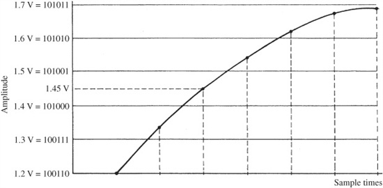
FIGURE 2.5 Quantization error is limited to one-half of the least significant bit.

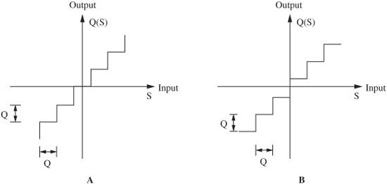
FIGURE 2.6 Signals can be quantized in one of two ways. A. A midtread quantizer. B. A midrise quantizer. Q (or 1 LSB) is the quantizer step size.

Generally, uniform step-size quantization is accomplished in one of two ways, as shown in the staircase functions in Fig. 2.6. Both methods provide equal numbers of positive and negative quantization levels. A midtread quantizer (Fig. 2.6A) places one quantization level at zero (yielding an odd number of steps or 2ⁿ − 1 where n is the number of bits); this architecture is generally preferred in many converters. A midrise quantizer (Fig. 2.6B), with an even number of steps 2n, does not have a quantization level at zero. A/D converter architecture is described in Chap. 3.

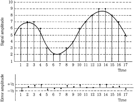
FIGURE 2.7 The amplitude value is rounded to the nearest quantization step. Quantization error at sample times is less than or equal to 1/2 LSB.

Quantization error is the difference between the actual analog value at sample time and the selected quantization interval value. At sample time, the amplitude value is rounded to the nearest quantization interval, as shown in Fig. 2.7. At best (sample points 11 and 12 in the figure), the waveform coincides with quantization intervals. At worst (sample point 1 in the figure), the waveform is exactly between two intervals. Quantization error is thus limited to a range between + Q/2 and − Q/2, where Q is one quantization interval (or 1 LSB). Note that this selection process, of one level or another, is the basic mechanism of quantization, and occurs for all samples in a digital system. Moreover, the magnitude of the error is always less than or equal to 1/2 LSB. This error results in distortion that is present for an audio signal of any amplitude. When the signal is large, the distortion is proportionally small and likely masked. However, when the signal is small, the distortion is proportionally large and might be audible.

In characterizing digital hardware performance, we can determine the ratio of the maximum expressible signal amplitude to the maximum quantization error; this determines the signal-to-error (S/E) ratio of the system. The S/E ratio of a digital system is similar, but not identical to the signal-to-noise (S/N) ratio of an analog system. The S/E relationship can be derived using a ratio of S/E voltage levels.

Consider a quantization system in which n is the number of bits, and N is the number of quantization steps. As noted:

N = 2ⁿ

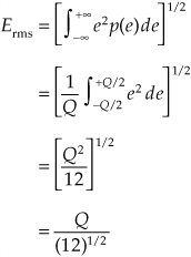
Half of these 2ⁿ values are used to code each part of the bipolar waveform. If Q is the quantizing interval, the peak values of the maximum signal levels are ±Q2ⁿ⁻¹. Assuming a sinusoidal input signal, the maximum root mean square (rms) signal S_rms is:

The energy of the quantization error can also be determined. When the input signal has high amplitude and wide spectrum, the quantization error is statistically independent and uniformly distributed between the + Q/2 and − Q/2 limits, and zero elsewhere, where Q is one quantization interval. This dictates a uniform probability density function with amplitude of 1/Q; the error is random from sample to sample, and the error spectrum is flat. Ignoring error outside the signal band, the rms quantization error E_rms can be found by summing (integrating) the product of the error and its probability:

The power ratio determining the signal to quantization error is:

Expressing this ratio in decibels:

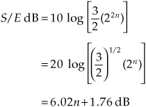
Using this approximation, we observe that each additional bit increases the S/E ratio (that is, reduces the quantization error) by about 6 dB, or a factor of two. For example, 16-bit quantization ideally yields an S/E ratio of about 98 dB, but 15-bit quantization is inferior at 92 dB. Looked at in another way, when the word length is increased by one bit, the number of quantization intervals is doubled. As a result, the distance between quantization intervals is halved, so the amplitude of the quantization error is also halved. Longer word lengths increase the data signal bandwidth required to convey the signal. However, the signal-to-quantization noise power ratio increases exponentially with data signal bandwidth. This is an efficient relationship that approaches the theoretical maximum, and it is a hallmark of coded systems such as pulse-code modulation (PCM) described in Chap. 3. The value of 1.76 is based on the statistics (peak-to-rms ratio) of a full-scale sine wave of peak amplitude; it will differ if the signal’s peak-to-rms ratio is different from that of a sinusoid.

It also is important to note that this result assumes that the quantization error is uniformly distributed, and quantization is accurate enough to prevent signal correlation in the error waveform. This is generally true for high-amplitude complex audio signals where the complex distortion components are uncorrelated, spread across the audible range, and perceived as white noise. However, this is not the case for low-amplitude signals, where distortion products can appear.

Quantization Error

Analysis of the quantization error of low-amplitude signals reveals that the spectrum is a function of the input signal. The error is not noise-like (as with high-amplitude signals); it is correlated. At the system output, when the quantized sample values reconstruct the analog waveform, the in-band components of the error are contained in the output signal. Because quantization error is a function of the original signal, it cannot be described as noise; rather, it must be classified as distortion.

As noted, when quantization error is random from sample to sample, the rms quantization error E_rms = Q/(12)^1/2. This equation demonstrates that the magnitude of the error is independent of the amplitude of the input signal, but depends on the size of the quantization interval; the greater the number of intervals, the lower the distortion. However, the relevant number of intervals is not only the number of intervals in the quantizer, but also the number of intervals used to quantize a particular signal. A maximum peak-to-peak signal (as used in the preceding analysis) presents the best case scenario because all the quantization intervals are exercised. However, as the signal level decreases, fewer and fewer levels are exercised, as shown in Fig. 2.8. For example, given a 16-bit quantizer, a half-amplitude signal would be mapped into half of the intervals. Instead of 65,536 levels, it would see 32,768 intervals. In other words, it would be quantized with 15-bit resolution.

The problem increases as the signal level decreases. A very low-level signal, for example, might receive only single-bit quantization or might not be quantized at all. In other words, as the signal level decreases, the percentage of distortion increases. Although the distortion percentage might be extremely small with a high level, 0 dBFS (dB Full Scale) signal, its percentage increases significantly at low-amplitude, for example, −90 dBFS levels. As described in a following section, dither must be used to alleviate the problem.

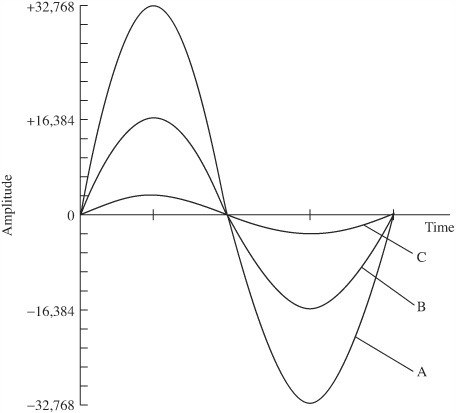
FIGURE 2.8 The percentage of quantization error increases as the signal level decreases. Full-scale waveform A has relatively low error (16-bit resolution). Half-scale waveform B has higher error (effectively 15-bit resolution). Low-amplitude waveform C has very high error.

The error floor of a digital audio system differs from the noise floor of an analog system because in a digital system the error is a function of the signal. The nature of quantization error varies with the amplitude and nature of the audio signal. For broadband, high-amplitude input signals (such as are typically found in music), the quantization error is perceived similarly to white noise. A high-level complex signal may show a pattern from sample to sample; however, its quantization error signal shows no pattern from sample to sample. The quantization error is thus independent of the signal (and thus assumes the characteristics of noise) when the signal is high level and complex. The only difference between this error noise and analog noise is that the range of values is more limited for a constant rms value. In other words, all values are equally likely to fall between positive and negative peaks. On the other hand, analog noise is Gaussian-distributed, so its peaks are higher than its rms value.

However, the perceptual qualities of the error are less benign for low-amplitude signals and high-level signals of very narrow bandwidth. This is based on the fact that white noise is perceptually benign because successive values of the signal are random, whereas predictable noise signals are more readily perceived. For broadband high-level signals, the statistical correlation between successive samples is very low; however, it increases for broadband low-level signals and narrow bandwidth, high-level signals. As the statistical correlation between samples increases, error initially perceived as benign white noise become more complex, yielding harmonic and intermodulation distortion as well as signal-dependent modulation of the noise floor.

Quantization distortion can take many guises. For example, the quantized signal might contain components above the Nyquist frequency; thus, aliasing might occur. The components appear after the sampler, but are effectively sampled. The effects of sampling the output of a limiter or limiting the output of a sampler are indistinguishable. If the signal is high level or complex, the alias components will add to the other complex, noise-like errors. If the input signal is low level and simple, the aliased components might be quite audible. Consider a system with sampling frequency of 48 kHz, bandlimited to 24 kHz. When a 5-kHz sine wave of amplitude of one quantizing step is applied, it is quantized as a sampled 5-kHz square wave. Harmonics of the square wave appear at 15, 25, and 35 kHz. The latter two alias back to 23 and 13 kHz, respectively. Other harmonics and aliases appear as well.

The aliasing caused by quantization can create an effect called granulation noise, so called because of its gritty sound quality. With high-level signals, the noise is masked by the signal itself. However, with low-level signals, the noise is audible. This blend of gritty, modulating noise and distortion has no analog counterpart and is audibly unpleasant. Furthermore, if the alias components are near a multiple of the sampling frequency, beat tones can be created, producing an odd sound called “bird singing” or “birdies.” A decaying tone presents a waveform descending through quantization levels; the error is perceptually changed from white noise to discrete distortion components. The problem is aggravated because even complex musical tones become more sinusoidal as they decay. Moreover, the decaying tone will tend to amplitude-modulate the distortion components. Dither addresses these quantization problems.

Other Architectures

Quantization is more than just word length; it also is a question of hardware architecture. There are many techniques for assigning quantization levels to analog signals. For example, a quantizer can use either a linear or nonlinear distribution of quantization intervals along the amplitude scale. One alternative is delta modulation, in which a one-bit quantizer is used to encode amplitude, using the single bit as a sign bit. In other cases, oversampling and noise shaping can be used to shift quantization error out of the audio band. Those algorithm decisions influence the efficiency of the quantizing bits, as well as the relative audibility of the error. For example, as noted, a linear quantizer produces a relatively high error with low-level signals that span only a few intervals. A nonlinear system using a floating point converter can increase the amplitude of low-level signals to utilize the greatest possible interval span. Although this improves the overall S/E ratio, the noise modulation by-product might be undesirable. Historically, after examining the trade-offs of different quantization systems, manufacturers determined that a fixed, linear quantization scheme is highly suitable for music recording. However, newer low bit-rate coding systems challenge this assumption. Alternative digitization systems are examined in Chap. 4. Low bit-rate coding is examined in Chaps. 10 and 11.

Dither

With large-amplitude complex signals, there is little correlation between the signal and the quantization error; thus, the error is random and perceptually similar to analog white noise. With low-level signals, the character of the error changes as it becomes correlated to the signal, and potentially audible distortion results. A digitization system must suppress any audible qualities of its quantization error. Obviously, the number of bits in the quantizing word can be increased, resulting in a decrease in error amplitude of 6 dB per additional bit. This is uneconomical because relatively many bits are needed to satisfactorily reduce the audibility of quantization error. Moreover, the error will always be relatively significant with low-level signals.

Dither is a far more efficient technique. Dither is a small amount of noise that is uncorrelated with the audio signal. Dither is added to the audio signal prior to sampling. This linearizes the quantization process. With dither, the audio signal is made to shift with respect to quantization levels. Instead of periodically occurring quantization patterns in consecutive waveforms, each cycle is different. Quantization error is thus decorrelated from the signal and the effects of the quantization error are randomized to the point of elimination. However, although it greatly reduces distortion, dither adds some noise to the output audio signal. When properly dithered, the number of bits in a quantizer determines the signal’s noise floor, but does not limit its low-level detail. For example, signals at −120 dBFS can be heard and measured in a dithered 16-bit recording.

Dither does not mask quantization error; rather, it allows the digital system to encode amplitudes smaller than the least significant bit, in much the same way that an analog system can retain signals below its noise floor. A properly dithered digital system far exceeds the signal to noise performance of an analog system. On the other hand, an undithered digital system can be inferior to an analog system, particularly with low-level signals. High-quality digitization demands dithering at the A/D converter. In addition, digital computations should be digitally dithered to alleviate requantization effects.

Consider the case of an audio signal with amplitude of two quantization intervals, as shown in Fig. 2.9A. Quantization yields a coarsely quantized waveform, as shown in Fig. 2.9B. This demonstrates that quantization ultimately acts as a hard limiter; in other words, severe distortion takes place. The effect is quite different when dither is added to the audio signal. Figure 2.9C shows a dither signal with amplitude of one quantization interval added to the input audio signal. Quantization yields a pulse signal that preserves the information of the audio signal, shown in Fig. 2.9D. The quantized signal switches up and down as the dithered input varies, tracking the average value of the input signal.

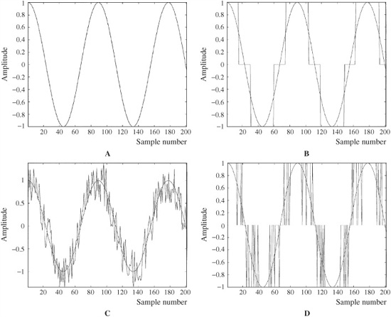
FIGURE 2.9 Dither is used to alleviate the effects of quantization error. A. An undithered input sine wave signal with amplitude of two LSBs. B. Quantization results in a coarse coding over three levels. C. Dither is added to the input sine wave signal. D. Quantization yields a PWM waveform that codes information below the LSB.

Low-level information is encoded in the varying width of the quantized signal pulses. This encoding is known as pulse-width modulation, and it accurately preserves the input signal waveform. The average value of the quantized signal moves continuously between two levels, alleviating the effects of quantization error. Similarly, analog noise would be coded as a binary noise signal; values of 0 and 1 would appear in the LSB in each sampling period, with the signal retaining its white spectrum. The perceptual result is the original signal with added noise—a more desirable result than a quantized square wave.

Mathematically, with dither, quantization error is no longer a deterministic function of the input signal, but rather becomes a zero-mean random variable. In other words, rather than quantizing only the input signal, the dither noise and signal are quantized together, and this randomizes the error, thus linearizing the quantization process. This particular technique is known as nonsubtractive dither because the dither signal is permanently added to the audio signal; the total error is not statistically independent of the audio signal, and errors are not independent sample to sample. However, nonsubtractive dither techniques do manipulate the statistical properties of the quantizer, statistically rendering conditional moments of the total error independent of the input, effectively decorrelating the quantization error of the samples from the signal, and from each other. The power spectrum of the total error signal can be made white. Subtractive dithering, in which the dither signal is removed after requantization, theoretically provides total error statistical independence, but is more difficult to implement.

John Vanderkooy and Stanley Lipshitz demonstrated the remarkable benefit of dither with a 1-kHz sine wave with a peak-to-peak amplitude of about 1 LSB, as shown in Fig. 2.10. Without dither, a square wave is output (Fig. 2.10A). When wideband Gaussian dither with an rms amplitude of about 1/3 LSB is added to the original signal before quantization, a pulse-width-modulated (PWM) waveform results (Fig. 2.10B). The encoded sine wave is revealed when the PWM waveform is averaged 32 times (Fig. 2.10C) and 960 times (Fig. 2.10D). The averaging illustrates how the ear responds in its perception of acoustic signals; that is, the ear is a lowpass filter that averages signals. In this case, a noisy sine wave is heard, rather than a square wave.

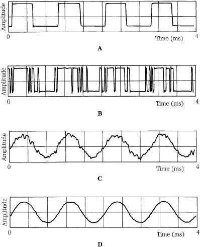
FIGURE 2.10 Dither permits encoding of information below the least significant bit. A. Quantizing a 1-kHz sine wave with peak-to-peak amplitude of 1 LSB without dither produces a square wave. B. Dither of 1/3 LSB rms amplitude is added to the sine wave before quantization, resulting in PWM modulation. C. Modulation conveys the encoded sine wave information, as can be seen after 32 averagings. D. The encoded sine wave information is more apparent after 960 averagings. (Vanderkooy and Lipshitz, 1984)

The ear is quite good at resolving narrow-band signals below the noise floor because of the averaging properties of the basilar membrane. The ear behaves as a one-third octave filter with a narrow bandwidth; the quantization error, which is given a white noise character by dither, is averaged by the ear, and the original narrow-band sine-wave is heard without distortion. In other words, dither changes the digital nature of the quantization error into white noise, and the ear can then resolve signals with levels well below one quantization level.

This conclusion is an important one. With dither, the resolution of a digitization system is far below the least significant bit; theoretically, there is no limit to the low-level resolution. By encoding the audio signal with dither to modulate the quantized signal, that information can be recovered, even though it is smaller than the smallest quantization interval. Furthermore, dither can eliminate distortion caused by quantization by reducing those artifacts to white noise. Proof of this is shown in Fig. 2.11, illustrating a computer simulation performed by John Vanderkooy, Robert Wannamaker, and Stanley Lipshitz. The figure shows a 1-kHz sine wave of 4 LSB peak-to-peak amplitude. The first column shows the signal without dither. The second column shows the same signal with triangular probability density function dither (explained in the following paragraphs) of 2 LSB peak-to-peak amplitude. In both cases, the first row shows the input signal. The second row shows the output signal. The third row shows the total quantization error signal. The fourth row shows the power spectrum of the output signal (this is estimated from sixty 50% overlapping Hann-windowed 512-point records at 44.1 kHz). The undithered output signal (Fig. 2.11D) suffers from harmonic distortion, visible at multiples of the input frequency, as well as inharmonic distortion from aliasing. The error signal (Fig. 2.11G) of the dithered signal shows artifacts of the input signal; thus, it is not statistically independent. Although it clearly does not look like white noise, this error signal sounds like white noise and the output signal sounds like a sine wave with noise. This is supported by the power spectrum (Fig. 2.11H) showing that the signal is free of signal-dependent artifacts, with a white noise floor. The highly correlated truncation distortion of undithered quantization is eliminated. However, we can see that dither increases the noise floor of the output signal.

Types of Dither

There are several types of dither signals, generally differentiated by their probability density function (pdf). Given a random signal with a continuum of possible values, the integral of the probability density function describes the probability of the values over an interval. The probability of where the dither signal falls within an interval defines the area under the function. For example, the dither signal might have equal probability of falling anywhere over an interval, or it might be more likely that the dither signal is in the middle of the interval. An interval, for example, might be 1 or 2 LSBs wide. For audio applications, interest has focused on three dither signals: Gaussian pdf, rectangular (or uniform) pdf, and triangular pdf, as shown in Fig. 2.12. For example, we might speak of a statistically independent, white dither signal with a triangular pdf having a peak-to-peak level or width of 2 LSB. Figure 2.13 shows how triangular pdf dither of 2-LSB peak-to-peak level would be placed in a midrise quantizer.

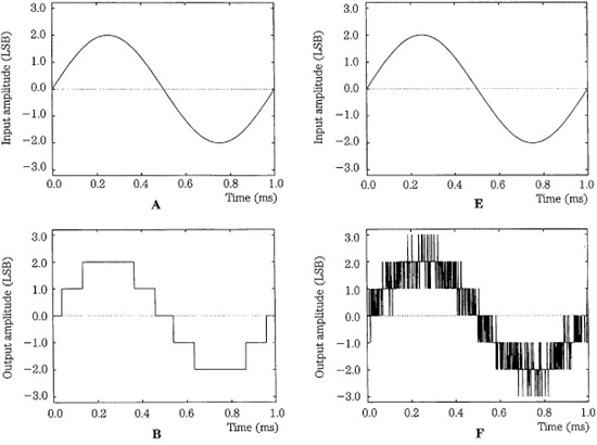
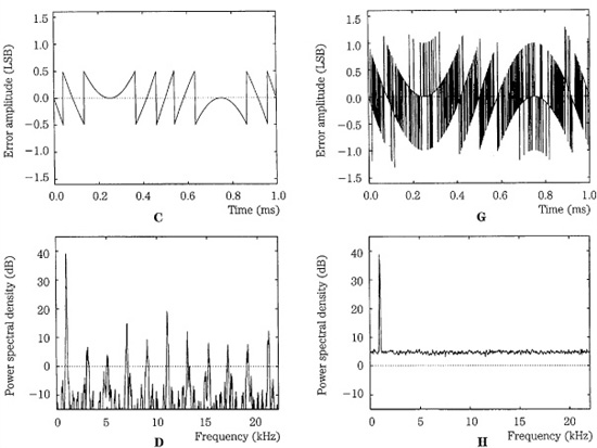
FIGURE 2.11 Computer-simulated quantization of a low-level 1-kHz sine wave without and with dither. A. Input signal. B. Output signal (no dither). C. Total error signal (no dither). D. Power spectrum of output signal (no dither). E. Input signal. F. Output signal (triangular dither). G. Total error signal (triangular dither). H. Power spectrum of output signal (triangular dither). (Lipshitz, Wannamaker, and Vanderkooy, 1992)

FIGURE 2.12 Probability density functions are used to describe dither signals. A. Rectangular pdf dither. B. Triangular pdf dither. C. Gaussian pdf dither.

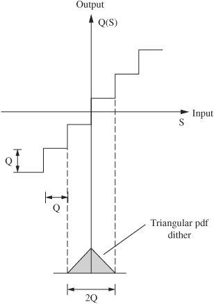
FIGURE 2.13 Triangular pdf dither of 2-LSB peak-to-peak level is placed at the origin of a midrise quantizer.

Dither signals may have a white spectrum. However, for some applications, the spectrum can be shaped by correlating successive dither samples without modifying the pdf; for example, a highpass triangular pdf dither signal could easily be created. By weighting the dither to higher frequencies, the audibility of the noise floor can be reduced.

All three dither types are effective at linearizing the transfer characteristics of quantization, but differ in their results. In almost all applications, triangular pdf dither is preferred. Rectangular and triangular pdf dither signals add less overall noise to the signal, but Gaussian dither is easier to implement in the analog domain.

Gaussian dither is easy to generate with common analog techniques; for example, a diode can be used as a noise source. The dither noise must vary between positive and negative values in each sampling period; its bandwidth must be at least half the sampling frequency. Gaussian dither with an rms value of 1/2 LSB will essentially linearize quantization errors; however, some noise modulation is added to the audio signal. The undithered quantization noise power is Q²/12 (or Q/(12)^1/2 rms), where Q is 1 LSB. Gaussian dither contributes noise power of Q²/4 so that the combined noise power is Q²/3 (or Q/(3)^1/2 rms). This increase in noise floor is significant.

Rectangular pdf dither is a uniformly distributed random voltage over an interval. Rectangular pdf dither lying between ±1/2 LSB (that is, a noise signal having a uniform probability density function with a peak-to-peak width that equals 1 LSB) will completely linearize the quantization staircase and eliminate distortion products caused by quantization. However, rectangular pdf does not eliminate noise floor modulation. With rectangular pdf dither, the noise level is more apt to be dependent on the signal, as well as width of the pdf. This noise modulation might be objectionable with very low frequencies or dynamically varied signals. If rectangular pdf dither is used, to be at all effective, its width must be an integer multiple of Q. Rectangular pdf dither of ± Q/2 adds a noise power of Q²/12 to the quantization noise of Q²/12; this yields a combined noise power of Q²/6 (or Q/(6)^1/2 rms).

It is believed that the optimal nonsubtractive dither signal is a triangular pdf dither of 2 LSB peak-to-peak width, formed by summing (convolving the density functions) of two independent rectangular pdf dither signals each 1 LSB peak-to-peak width. Triangular pdf dither eliminates both distortion and noise floor modulation. The noise floor is constant; however, the noise floor is higher than in rectangular pdf dither. Triangular pdf dither adds a noise power of Q²/6 to the quantization noise power of Q²/12; this yields a combined noise power of Q²/4 (or Q/2 rms). The AES17 standard specifies that triangular pdf dither be used when evaluating audio systems. Because all analog signals already contain Gaussian noise that acts as dither, A/D converters do not necessarily use triangular pdf dither. In some converters, Gaussian pdf dither is applied.

Using optimal dither amplitudes, relative to a nondithered signal, rectangular pdf dither increases noise by 3 dB, triangular pdf dither increases noise by 4.77 dB, and Gaussian pdf dither increases noise by 6 dB. In general, rectangular pdf is sometimes used for testing purposes because of its expanded S/E ratio, but triangular pdf is far preferable for most applications including listening purposes, in spite of its slightly higher noise floor. Clearly, Gaussian dither has a noise penalty. Because rectangular and triangular pdf dither are easily generated in the digital domain, they are always preferable to Gaussian dither in requantization applications prior to D/A conversion. When measuring the low-level distortion of digital audio products, it is important to use dithered test signals; otherwise, the measurements might reflect distortion that is an artifact of the test signal and not of the hardware under test. However, a dithered test signal will limit measured noise level and distortion performance. In practical use, analog audio signals contain thermal (Gaussian) noise; even when otherwise theoretically optimal dither is added, nonoptimal results are obtained.

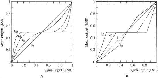
FIGURE 2.14 Input/output transfer characteristic showing the effects of dither of varying amplitudes. A. Gaussian pdf dither of 1/2 LSB rms linearizes the audio signal. B. Rectangular pdf dither of 1 LSB linearizes the audio signal. (Vanderkooy and Lipshitz, 1984)

The amplitude of any dither signal is an important concern. Figure 2.14 shows how a quantization step is linearized by adding different amplitudes (width of pdf) of Gaussian pdf and rectangular pdf dither. In both cases, quantization artifacts are decreased as relatively higher amplitudes of dither are added. As noted, a Gaussian pdf signal with an amplitude of 1/2 LSB rms provides a linear characteristic. With rectangular pdf dither, a level of 1 LSB peak-to-peak provides linearity. In either case, too much dither overly decreases the S/N ratio of the digital system with no additional benefit.

The increase in noise yielded by dither is usually negligible given the large S/E ratio inherent in a digital system, and its audibility can be minimized, for example, with a highpass dither signal. This can be easily accomplished with digitally generated dither. For example, the spectrum of a triangular pdf dither can be processed so that its amplitude rises at high audio frequencies. Because the ear is relatively insensitive to high frequencies, this dither signal will be less audible than broadband dither, yet noise modulation and signal distortion are removed. Such techniques can be used to audibly reduce quantization error, for example, when converting a 20-bit signal to a 16-bit signal. More generally, signal processing can be used to psychoacoustically shape the quantization noise floor to reduce its audibility. Noise-shaping applications are discussed in Chap. 18.

Designers have observed that the amplitude of a dither signal can be decreased if a sine wave with a frequency just below the Nyquist frequency, with an amplitude of 1 or 1/2 quantization interval, is added to the audio signal. The added signal must be above audibility yet below the Nyquist frequency to prevent aliasing. It alters the spectrum of quantization error to minimize its audibility and overall does not add as much noise to the signal as broadband dither. For example, discrete triangular pdf dither might yield a 2-dB penalty, as opposed to 4.77 dB. However, a discrete dither frequency might lead to intermodulation products with audio signals. Wideband dither signals alleviate this artifact.

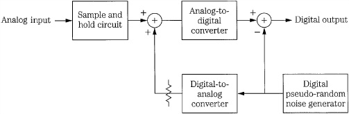
FIGURE 2.15 An example of a subtractive digital dither circuit using a pseudo-random number generator. (Blesser, 1983)

An additive dither signal necessarily decreases the S/E ratio of the digitization system. A subtractive dither signal proposed by Barry Blesser that would preserve the S/E ratio is shown in Fig. 2.15. Rectangular noise is a random-valued signal that can be simulated by generating a quickly changing pseudo-random sequence of digital data. This can be accomplished with a series of shift registers and a feedback network comprising exclusive or gates. This sequence is input to a D/A converter to produce analog noise which is added to the audio signal to achieve the benefit of dither. Then, following A/D conversion, the dither is digitally subtracted from the audio signal, preserving the dynamic range of the original signal. A further benefit is that inaccuracies in the A/D converter are similarly randomized. Other additive-subtractive methods call for two synchronized pseudo-random signal generators, one adding rectangular pdf dither at the A/D converter, and the other subtracting it at the D/A converter. Alternatively, in an auto-dither system, the audio signal itself could be randomized to create an added dither at the A/D converter, then re-created at the D/A converter and subtracted from the audio signal to restore the dynamic range.

Digital dither must be used to decrease distortion and artifacts created by round-off error when signal manipulation takes place in the digital domain. For example, the truncation associated with multiplication can cause objectionable error. Digital dither is described in Chap. 17.

For the sake of completeness, and although the account is difficult to verify, one of the early uses of dither came in World War II. Airplane bombers used mechanical computers to perform navigation and bomb trajectory calculations. Curiously, these computers (boxes filled with hundreds of gears and cogs) performed more accurately when flying on board the aircraft, and less well on terra firma. Engineers realized that the vibration from the aircraft reduced the error from sticky moving parts. Instead of moving in short jerks, they moved more continuously. Small vibrating motors were built into the computers, and their vibration was called dither from the Middle English verb “didderen,” meaning “to tremble.” Today, when you tap a mechanical meter to increase its accuracy, you are applying dither, and dictionaries define dither as “a highly nervous, confused, or agitated state.” At any rate, in minute quantities, dither successfully makes a digitization system a little more analog in the good sense of the word.

Summary

Sampling and quantizing are the two fundamental elements of an audio digitization system. The sampling frequency determines signal bandlimiting and thus frequency response. Sampling is based on well-understood principles; the cornerstone of discrete-time sampling yields completely predictable results. Aliasing can occur when the sampling theorem is not observed. Quantization determines the dynamic range of the system, measured by the S/E ratio. Although bandlimited sampling is a lossless process, quantization is one of approximation. Quantization artifacts can severely affect the performance of a system. However, dither can eliminate quantization distortion, and maintain the fidelity of the digitized audio signal. In general, a sampling frequency of 44.1 kHz or 48 kHz and a dithered word length of 16 to 20 bits yields fidelity comparable to or better than the best analog systems, with advantages such as longevity and fidelity of duplication. Still higher sampling frequencies and longer word lengths can yield superlative performance. For example, a sampling frequency of 192 kHz and a word length of 24 bits is available in the Blu-ray disc format.

Postscript

A special note on high sampling frequencies: Before ending our discussion of discrete time sampling, consider a hypothesis concerning the nature of time. Time seems to be continuous. However, physicists have suggested that, just as this book consists of a finite number of atoms, time might come in discrete intervals. Specifically, the indivisible period of time might be 10⁻⁴³ second, known as Planck time. One theory is that no time interval can be shorter than this because the energy required to make the division would be so great that a black hole would be created and the event would be swallowed up inside it. If any of you are experimenting in your basements with very high sampling frequencies, please be careful.