Budgeting the Project

Having finished the planning for the technical aspects of the project, there is one more important element of planning to finish that will then result in the final go-ahead from top management to initiate the project. A budget must be developed in order to obtain the resources needed to accomplish the project's objectives. A budget is simply a plan for allocating organizational resources to the project activities. PMBOK covers the topic of budgeting in Chapter 7 on Cost.

But the budget also serves another purpose: It ties the project to the organization's aims and objectives through organizational policy. For example, NASA's Mars Pathfinder-Rover mission embedded a new NASA policy—to achieve a set of limited exploration opportunities at extremely limited cost. In 1976, NASA's two Viking-Mars Lander missions cost $3 billion to develop. In 1997, however, the Pathfinder-Rover mission cost only $175 million to develop, a whopping 94 percent reduction. The difference was the change in organizational policy from a design-to-performance orientation to a design-to-cost orientation.

In Chapter 3, we described the project planning process as a set of steps that began with the overall project plan and then divided and subdivided the plan's elements into smaller and smaller pieces that could finally be sequenced, assigned, scheduled, and budgeted. Hence, the project budget is nothing more than the project plan, based on the WBS, expressed in monetary terms and it becomes a part of the Project Charter.

Once the budget is developed, it acts as a tool for upper management to monitor and guide the project. As we will see later in this chapter, it is a necessary managerial tool, but it is not sufficient. Appropriate data must be collected and accurately reported in a timely manner or the value of the budget to identify current financial problems or anticipate upcoming ones will be lost. This collection and reporting system must be as carefully designed as the initial project plans because late reporting, inaccurate reporting, or reporting to the wrong person will negate the main purpose of the budget. In one instance, the regional managers of a large computer company were supposed to receive quarterly results for the purpose of correcting problems in the following quarter. The results took 4 months to reach them, however, completely negating the value of the budgeting-reporting system.

In this chapter, we will first examine some different methods of budgeting and cost estimating, as used for projects. Then we will consider some ways to improve the cost estimation process, including some technical approaches such as learning curves and tracking signals. We will also discuss some ways to misuse the budget that are, unfortunately, common. Last, we discuss the problem of budget uncertainty and the role of risk management when planning budgets.

4.1 METHODS OF BUDGETING

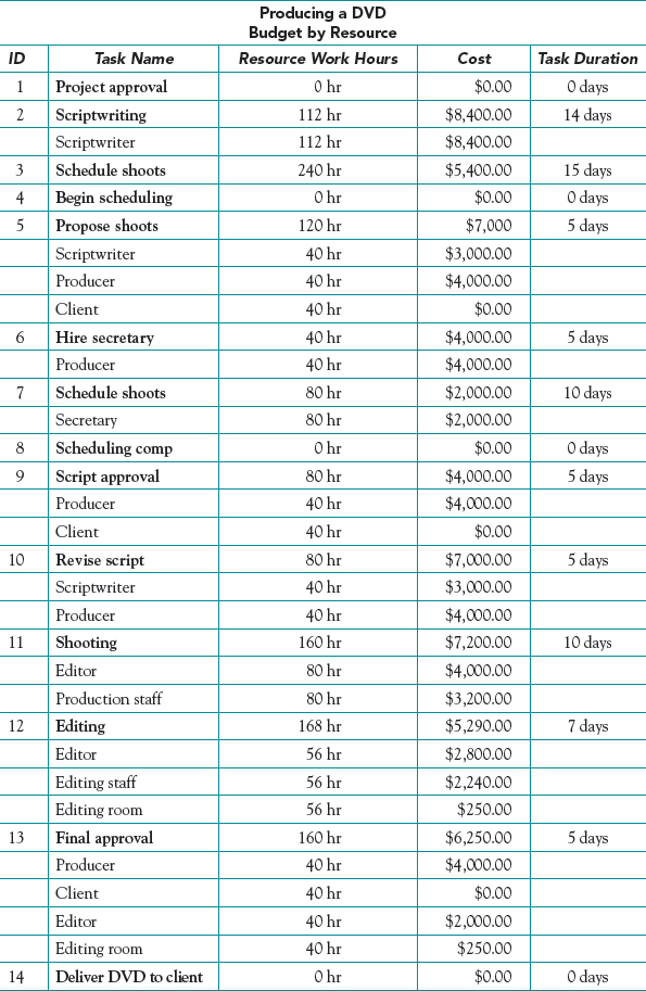
Budgeting is simply the process of forecasting what resources the project will require, what quantities of each will be needed, when they will be needed, and how much they will cost. Tables 4-1 and 4-2 depict the direct costs involved in making a short documentary film. Table 4-1 shows the cost per unit of usage (cost/hour) of seven different personnel categories and one facility. Note that the facility does not charge by the hour, but has a flat rate charge. Table 4-2 shows the resource categories and amounts used for each activity required to make the DVD. The resource costs shown become part of the budget for producing the documentary film. As you will see below, overhead charges may be added to these direct charges.

Most businesses and professions employ experienced estimators who can forecast resource usage with amazingly small errors. For instance, a bricklayer can usually estimate within 1 or 2 percent the number of bricks required to construct a brick wall of given dimensions. In many fields, the methods of cost estimation are well documented based on the experience of estimators gathered over many years. The cost of a building, or house, is usually estimated by the square feet of floor area multiplied by an appropriate dollar value per square foot and then adjusted for any unusual factors.

Budgeting a project such as the development of a control system for a new computer, however, is often more difficult than budgeting more routine activities—and even more difficult than regular departmental budgeting which can always be estimated as: “Same as last year plus X percent.” But project budgeters do not usually have tradition to guide them. Projects are, after all, unique activities. Of course, there may be somewhat similar past projects that can serve as a model, but these are rough guides at best. Forecasting a budget for a multiyear project such as a large product line or service development project is even more hazardous because the unknowns can escalate quickly with changes in technology, materials, prices, and even the findings of the project up to that point.

Table 4-1 Resource Cost per Unit for Producing a Short Documentary Film

Table 4-2 Budget by Resource for Producing a Short Documentary Film

Organizational tradition also impacts project budgeting. Every firm has its own rules about how overhead and other indirect costs are charged against projects. Every firm has its ethical codes. Most firms must comply with the Sarbanes-Oxley Act (SOX) and the Health Insurance Portability and Accountability Act (HIPAA). Most firms have their own accounting idiosyncrasies, and the PM cannot expect the accounting department to make special allowances for his or her individual project. Although accounting will charge normal expenditures against a particular activity's account number, as identified in the WBS, unexpected overhead charges, indirect expenses, and usage or price variances may suddenly appear when the PM least expects it, and probably at the worst possible time. (Price variances due to procurement, and the entire procurement process, are discussed in Chapter 12 of PMBOK, 2013.) There is no alternative—the PM must simply become completely familiar with the organization's accounting system, as painful as that may be.

In the process of gaining this familiarity, the PM will discover that cost may be viewed from three different perspectives (Hamburger, 1986). The PM recognizes a cost once a commitment is made to pay someone for resources or services, for example when a machine is ordered. The accountant recognizes an expense when an invoice is received—not, as most people believe, when the invoice is paid. The controller perceives an expense when the check for the invoice is mailed. The PM is concerned with commitments made against the project budget. The accountant is concerned with costs when they are actually incurred. The controller is concerned with managing the organization's cash flows. Because the PM must manage the project, it is advisable for the PM to set up a system that will allow him or her to track the project's commitments.

Another aspect of accounting that will become important to the unaware PM is that accountants live in a linear world. When a project activity has an $8,000 charge and runs over a four-month period, the accounting department (or worse, their software) sometimes simply spreads the $8,000 evenly over the time period, resulting in a $2,000 allocation per month. If expenditures for this activity are planned to be $5,000, $1,000, $1,000, and $1,000, the PM should not be surprised when the organization's controller storms into the project office after the first month screaming about the unanticipated and unacceptable cash flow demands of the project!

Next, we look at two different approaches for gathering the data for budgeting a project: top-down and bottom-up.

Top-down Budgeting

The top-down approach to budgeting is based on the collective judgments and experiences of top and middle managers concerning similar past projects. These managers estimate the overall project cost by estimating the costs of the major tasks, which estimates are then given to the next lower level of managers to split up among the tasks under their control, and so on, until all the work is budgeted.

The advantage of this approach is that overall budget costs can be estimated with fair accuracy, though individual elements may be in substantial error. Another advantage is that errors in funding small tasks need not be individually identified because the overall budget allows for such exceptions. Similarly, the good chance that some small but important task was overlooked does not usually cause a serious budgetary problem. The experience and judgment of top management are presumed to include all such elements in the overall estimate. In the next section, we will note that the assumptions on which these advantages are based are not always true.

Bottom-Up Budgeting

In bottom-up budgeting, the WBS identifies the elemental tasks, whose resource requirements are estimated by those responsible for executing them (e.g., programmer-hours in a software project). This can result in much more accurate estimates, but it often does not do so for reasons we will soon discuss. The resources, such as labor and materials, are then converted to costs and aggregated to different levels of the project, eventually resulting in an overall direct cost for the project. The PM then adds, according to organizational policy, indirect costs such as general and administrative, a reserve for contingencies, and a profit figure to arrive at a final project budget.

Bottom-up budgets are usually more accurate in the detailed tasks, but risk the chance of overlooking some small but costly tasks. Such an approach, however, is common in organizations with a participative management philosophy and leads to better morale, greater acceptance of the resulting budget, and heightened commitment by the project team. It is also a good managerial training technique for aspiring project and general managers.

Unfortunately, true bottom-up budgeting is rare. Upper level managers are reluctant to let the workers develop the budget, fearing the natural tendency to overstate costs, and fearing complaints if the budget must later be reduced to meet organizational resource limitations. Moreover, the budget is upper management's primary tool for control of the project, and they are reluctant to let others set the control limits. Again, we will see that the budget is not a sufficient tool for controlling a project. Top-down budgeting allows the budget to be controlled by people who play little role in designing and doing the work required by the project. It should be obvious that this will cause problems—and it does.

We recommend that organizations employ both forms of developing budgets. They both have advantages, and the use of one does not preclude the use of the other. Making a single budget by combining the two depends on setting up a specific system to negotiate the differences. We discuss just such a system below. The only disadvantage of this approach is that it requires some extra time and trouble, a small price to pay for the advantages. A final warning is relevant. Any budgeting system will be useful only to the extent that all cost/revenue estimates are made with scrupulous honesty.

4.2 COST ESTIMATING

In this section, we look at the details of the process of estimating costs and some dangers of arbitrary cuts in the project budget. We also describe and illustrate the difference between activity budgeting and program budgeting.

Work Element Costing

The task of building a budget is relatively straightforward but tedious. Each work element is evaluated for its resource requirements, and its costs are then determined. For example, suppose a certain task is expected to require 16 hours of labor at $10 per hour, and the required materials cost $235. In addition, the organization charges overhead for the use of utilities, indirect labor, and so forth at a rate of 50 percent of direct labor. Then, the total task cost will be

$235 + [(16 hr × $10/hr) × 1.5] = $475

In some organizations, the PM adds the overhead charges to the budget. In others, the labor time and materials are just sent to the accounting department and they run the numbers, add the appropriate overhead, and total the costs. Although overhead was charged here against direct labor, more recent accounting practices such as activity-based costing may charge portions of the overhead against other cost drivers such as machine time, weight of raw materials, or total time to project completion.

Direct resource costs such as for materials and machinery needed solely for a particular project are usually charged to the project without an overhead add-on. If machinery from elsewhere in the organization is used, this may be charged to the project at a certain rate (e.g., $/hr) that will include depreciation charges, and then will be credited to the budget of the department owning and paying for the machine. On top of this, there is often a charge for GS&A (general, sales, and administrative) costs that includes upper management, staff functions, sales and marketing, plus any other costs not included in the overhead charge. GS&A may be charged as a percentage of direct costs, all direct and indirect costs, or on other bases including total time to completion.

Thus, the fully costed task will include direct costs for labor, machinery, and resources such as materials, plus overhead charges, and finally, GS&A charges. The full cost budget is then used by accounting to estimate the profit to be earned by the project. The wise PM, however, will also construct a budget of direct costs for his or her own use. This budget provides the information required to manage the project without being confounded with costs over which he or she has no control.

Note that the overhead and GS&A effect can result in a severe penalty when a project runs late, adding significant additional and possibly unexpected costs to the project. Again, we stress the importance of the PM thoroughly understanding the organization's accounting system, and especially how overhead and other such costs are charged to the project.

Of course, this process can also be reversed to the benefit of the PM by minimizing the use of drivers of high cost. Sometimes clients will even put clauses in contracts to foster such behavior. For example, when the state of Pennsylvania contracted for the construction of the Limerick nuclear power generating facility in the late 1980s, they included such an incentive fee provision in the contract. This provision stated that any savings that resulted from finishing the project early would be split between the state and the contractor. As a result, the contractor went to extra expense and trouble to make sure the project was completed early. The project came in 8 months ahead of its 49-month due date and the state and the contractor split the $400 million savings out of the total $3.2 billion budget.

The Impact of Budget Cuts

In the previous chapter on planning, we described a process in which the PM plans Level 1 activities, setting a tentative budget and duration for each. Subordinates (and this term refers to anyone working on the project even though such individuals may not officially report to the PM and may be “above” the PM on the firm's organizational chart) then take responsibility for specifying the Level 2 activities required to produce the Level 1 task. As a part of the Level 2 specifications, tentative budgets and durations are noted for each Level 2 activity. The PM's initial budget and duration estimates are examples of top-down budgeting. The subordinate's estimates of the Level 2 task budgets and durations are bottom-up budgeting. As we promised, we now deal with combining the two budgets.

We will label the Level 1 task estimate of duration of the i^th task as t_i, and the respective cost estimate as r_i, the t standing for “time” and the r for “resources.” In the meantime, the subordinate has estimated task costs and durations for each of the Level 2 tasks that comprise Level 1 task i. We label the aggregate cost and duration of these Level 2 activities as r_i′ and t_i′, respectively. It would be nice if r_i, equaled r_i′, but the reality is rarely that neat. In general, r_i<<r_i′ (The same is true of the time estimates, t_i and t_i′.) There are three reasons why this happens. First, jobs always look easier, faster, and cheaper to the boss than to the person who has to do them (Gagnon and Mantel, 1987). Second, bosses are usually optimistic and never admit that details have been forgotten or that anything can or will go wrong. Third, subordinates are naturally pessimistic and want to build in protection for everything that might possibly go wrong.

It is important that we make an assumption for the following discussion. We assume that both boss and subordinate are reasonably honest. What follows is a win-win negotiation, and it will fail if either party is dishonest. (We feel it is critically important to remind readers that it is never smart to view the other party in a negotiation as either stupid or ignorant. Almost without fail, such thoughts are obvious to the other party and the possibility of a win-win solution is dead.) The first step in reducing the difference between the superior's and subordinate's estimates occurs when the worker explains the reality of the task to the boss, and r_i rises. Encouraged by the fact that the boss seems to understand some of the problems, the subordinate responds to the boss's request to remove some of the protective padding. The result is that r_i′ falls.

The conversation now shifts to the technology involved in the subordinate's work and the two parties search for efficiencies in the Level 2 work plan. If they find some, the two estimates get closer still, or, possibly, the need for resources may even drop below either party's estimate.

To complete our discussion, let's assume that after all improvements have been made, r_i′ is still somewhat higher than r_i. Should the boss accept the subordinate's cost estimate or insist that the subordinate accept the boss's estimate? To answer this question, we must recall the discussion of project life cycles from Chapter 1. We discussed two different common forms of life cycles, and these are illustrated again, for convenience, in Figure 4-1. One curve is S-shaped, and the other is J-shaped. As it happens, the shapes of these curves hold the key to our decision.

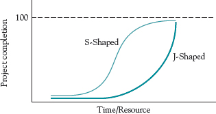
Figure 4-1 Two project life cycles (cf. Figures 1-2 and 1-3).

If the project life cycle is S-shaped, then with a somewhat reduced level of resources, a smaller than proportional cut will be made in the project's objectives or performance, likely not a big problem. If the project's life cycle is J-shaped, the impact of inadequate resources will be serious, a larger than proportional cut will be made in the project's performance. The same effect occurs during an “economy drive” when a senior manager decrees an across-the-board budget cut for all projects of, say, 5 or 10 percent. For a project with a J-shaped life cycle, the result is disaster. It is not necessary to know the actual shape of a project's life cycle with any precision. One needs merely to know the probable curvature (concave or convex to the baseline) of the last stage of the cycle for the project being considered.

The message here is that for projects with S-shaped life cycles, the top-down budgeting process is probably acceptable. For J-shaped life-cycle projects, it is dangerous for upper management not to accept the bottom-up budget estimates. At the very least, management should pay attention when the PM complains that the budget is insufficient to complete the project. An example of this problem is NASA's Space Shuttle Program, projected by NASA to cost $10-13 billion but cut by Congress to $5.2 billion. Fearing a cancellation of the entire program if they pointed out the overwhelming developmental problems they faced, NASA acquiesced to the inadequate budget. As a result, portions of the program fell 3 years behind schedule and had cost overruns of 60 percent. As the program moved into the operational flight stage, problems stemming from the inadequate budget surfaced in multiple areas, culminating in the Challenger explosion in January 1986.

Finally, in these days of increasing budget cuts and great stress on delivering project value, cuts to the organization's project portfolio must be made with care. Wheatly (2009) warns against the danger of focusing solely on ROI when making decisions about which projects will be kept and which will be terminated. We will have considerably more to say about this subject in Chapter 8.

An Aside

Here and elsewhere, we have preached the importance of managers and workers who are willing to communicate with one another frequently and honestly when developing budgets and schedules for projects. Such communication is the exception, not the rule. The fact that only a small fraction of software development projects are completed even approximately on time and on budget is so well known as to be legend, as is the record of any number of high technology industries. Sometimes the cause is scope creep, but top-down budgeting and scheduling are also prime causes. Rather than deliver another sermon on the subject, we simply reprint Rule #25 from an excellent book by Jim McCarthy, Dynamics of Software Development (1995).

Activity vs. Program Budgeting

Traditional organizational budgets are typically activity oriented and based on historical data accumulated through an activity-based accounting system. Individual expenses are classified and assigned to basic budget lines such as phone, materials, fixed personnel types (salaried, exempt, etc.), or to production centers or processes. These lines are then aggregated and reported by organizational units such as departments or divisions.

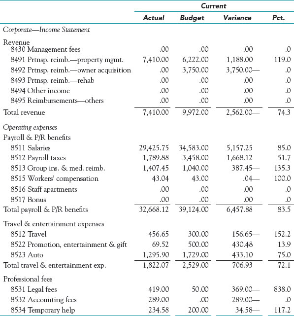
Project budgets can also be presented as activity budgets, such as in Table 4-3 where one page of a six-page monthly budget report for a real estate management project is illustrated. When multiple projects draw resources from several different organizational units, the budget may be divided between these multiple units in some arbitrary fashion, thereby losing the ability to control project resources as well as the reporting of individual project expenditures against the budget.

This difficulty gave rise to program budgeting, illustrated in Table 4-4. Here the program-oriented project budget is divided by task and expected time of expenditure, thereby allowing aggregation across projects. Budget reports are shown both aggregated and disaggregated by “regular operations,” and each of the projects has its own budget. For example, Table 4-3 would have a set of columns for regular operations as well as for each project.

Table 4-3 Typical Monthly Budget for a Real Estate Project (page 1 of 6)

4.3 IMPROVING COST ESTIMATES

At the end of his “Don't Accept Dictation,” reprinted above, McCarthy wrote “Each person who has a task to do must own the design and execution of that task and must be held accountable for its timely achievement. Accountability is the twin of empowerment.” If empowerment is to be trusted, it must be accompanied by accountability. Fortunately, it is not difficult to do this. This section deals with a number of ways for improving the process of cost estimating and an easy way of measuring its accuracy. These improvements are not restricted to cost estimates, but can be applied to almost all of the areas in project management that call for estimating or forecasting any aspect of a project that is measured numerically; e.g., task durations, the time for which specialized personnel will be required, or the losses associated with specific types of risks should they occur. These improvements range from better formalization of the estimating/forecasting process, using forms and other simple procedures, to straightforward quantitative techniques involving learning curves and tracking signals. We conclude with some miscellaneous topics, including behavioral issues that often lead to incorrect budget estimates.

Table 4-4 Project Budget by Task and Month

Forms

The use of simple forms such as that in Figure 4-2 can be of considerable help to the PM in obtaining accurate estimates, not only of direct costs, but also when the resource is needed, how many are needed, who should be contacted, and if it will be available when needed. The information can be collected for each task on an individual form and then aggregated for the project as a whole.

Learning Curves

Suppose a firm wins a contract to supply 25 units of a complex electronic device to a customer. Although the firm is competent to produce this device, it has never produced one as complex as this. Based on the firm's experience, it estimates that if it were to build many such devices it would take about 4 hours of direct labor per unit produced. With this estimate, and the wage and benefit rates the firm is paying, the PM can derive an estimate of the direct labor cost to complete the contract.

Unfortunately, the estimate will be in considerable error because the PM is underestimating the labor costs to produce the initial units that will take much longer than 4 hours each. Likewise, if the firm built a prototype of the device and recorded the direct labor hours, which may run as high as 10 hours for this device, this estimate applied to the contract of 25 units would give a result that is much too high.

In both cases, the reason for the error is the learning exhibited by humans when they repeat a task. In general, it has been found that unit performance improves by a fixed percent each time the total production quantity doubles. More specifically, each time the output doubles, the worker hours per unit decrease by a fixed percentage of their previous value. This percentage is called the learning rate, and typical values run between 70 and 95 percent. The higher values are for more mechanical tasks, while the lower, faster-learning values are for more mental tasks such as solving problems. A common rate in manufacturing is 80 percent. For example, if the device described in the earlier example required 10 hours to produce the first unit and this firm generally followed a typical 80 percent learning curve, then the second unit would require .80 × 10 = 8 hours, the fourth unit would require 6.4 hours, the eighth unit 5.12 hours, and so on. Of course, after a certain number of repetitions, say 100 or 200, the time per unit levels out and little further improvement occurs.

Figure 4-2 Form for gathering data on project resource needs.

Mathematically, this relationship we just described follows a negative exponential function. Using this function, the time required to produce the nth unit can be calculated as

T_n = T₁n^r

where T_n is the time required to complete the nth unit, T₁ is time required to complete the first unit, and r is the exponent of the learning curve and is calculated as the log(learning rate)/log(2). Tables are widely available for calculating the completion time of unit n and the cumulative time to produce units one through n for various learning rates; for example, see Meredith and Shafer (2013). The impact of learning can also be incorporated into spreadsheets developed to help prepare the budget for a project as is illustrated in the example at the end of this section.

The use of learning curves in project management has increased greatly in recent years. For instance, methods have been developed to approximate composite learning curves for entire projects (Amor and Teplitz, 1998), for approximating total costs from the unit learning curve (Camm, Evans, and Womer, 1987), and for including learning curve effects in critical resource diagramming (Badiru, 1995). The conclusion is that the effects of learning, even in “one-time” projects, should not be ignored. If costs are underestimated, the result will be an unprofitable project and senior management will be unhappy. If costs are overestimated, the bid will be lost to a savvier firm and senior management will be unhappy.

Tracking Signals

In Chapter 3, we noted that people do not seem to learn by experience, no matter how much they urge others to do so. PMs and others involved with projects spend much time estimating—activity costs and durations, among many other things. There are two types of error in those estimates. First, there is random error. Errors are random when there is a roughly equal chance that estimates are above or below the true value of a variable, and the average size of the error is approximately equal for over and under estimates. (Naturally, we try to devise ways of estimating that minimize the size of these random errors.) If either of the above is not true for an estimator—either the chance of over or under estimates are not about equal or the size of over or under estimates are not approximately equal—the estimates are said to be biased. Random errors cancel out, which means that if we add them up the sum will approach zero. Errors caused by bias do not cancel out. They are systematic errors.

Calculation of a number called the tracking signal can reveal if there is systematic bias in cost and other estimates and whether the bias is positive or negative. Knowing this can then be quite helpful to a PM in making future estimates or on the critically important task of judging the quality of estimates made by others. Consider the spreadsheet data in Figure 4-3 where estimated and actual values for some factor are listed in the order they were made, indicated for ease of reference by “period.” In order to compare estimates of different resources measured in units and of different magnitudes, we will derive a tracking signal based on the ratio of actual to estimated values rather than the usual difference between the two.

To calculate the first period ratio in Figure 4-3, for example, we would take the ratio 163/155 = 1.052. This means that the actual was 5.2 percent higher than the estimate, a forecast that was low. In column D, we list these errors for each of the periods and then cumulate them at the bottom of the spreadsheet. Note that in columns D and E we subtract 1 from the ratio. This centers the data around zero rather than 1.0, which makes some ratios positive, indicating an actual greater than the forecast, and other ratios negative, indicating an actual less than the forecast. If the cumulative percent error at the bottom of the spreadsheet is positive, which it is in this case, it means that the actuals are usually greater than the estimates. The forecaster underestimates if the ratio is positive and overestimates if it is negative. The larger the percent error, the greater the forecaster's bias, systematic under- or overestimation.

Figure 4-3 Excel^® template for finding bias in estimates.

Column E simply shows the absolute value of column D. Column F is the “mean absolute ratio,” abbreviated MAR, which is the running average of the values in column E up to that period. (Check the formulas in the spreadsheet of Figure 4-3.) The tracking signal listed in column G is the ratio of the running sum of the values in column D divided by the MAR for that period. If the estimates are unbiased, the running sum of ratios in column D will be about zero, and dividing this by the MAR will give a very small tracking signal, possibly zero. On the other hand, if there is considerable bias in the estimates, either positive or negative, the running sum of the ratios in column D will grow quite large. Then, when divided by the mean absolute ratio this will show whether the tracking signal is > 1 or < 1, and therefore greater than the variability in the estimates or not. If the bias is large, resulting in large positive or negative ratios, the resulting tracking signal will be correspondingly positive or negative.

It should be noted that it is not simply the bias that is of interest to the PM, although bias is very important. The MAR is also important because this indicates the variability of the estimates compared with the resulting actual values. With experience, the MAR should decrease over time though it will never reach zero. We strive to find a forecasting technique that minimizes both the bias and the MAR. By observing her own errors, the PM can learn to make unbiased estimates. When meeting with her subordinates in order to coach them on improving their estimates, it is important to recognize that most overestimates of duration or resource requirements are the result of an attempt by the subordinate to make “safe” estimates, and underestimates result from overoptimism. If subordinates overcorrect, the PM should avoid sharp criticism. Reasonable accuracy is the goal, but the uncertainty surrounding all projects does not allow random estimate errors to vanish.

Other Factors

Studies consistently show that between 60 and 85 percent of projects fail to meet their time, cost, and/or performance objectives. The record for information system (IS) projects is particularly poor, it seems. For example, there are at least 45 estimating models available for IS projects but few IS managers use any of them (Lawrence, 1994; Martin, 1994). While the variety of problems that can plague project cost estimates seem to be unlimited, there are some that occur with high frequency; we will discuss each of these in turn.

Changes in resource prices, for example, are a common problem. The most common managerial approach to this problem is to increase all cost estimates by some fixed percentage. A better approach, however, is to identify each input that has a significant impact on the costs and to estimate the rate of price change for each one. The Bureau of Labor Statistics (BLS) in the U.S. Department of Commerce publishes price data and “inflators” (or “deflators”) for a wide range of commodities, machinery, equipment, and personnel specialities. (For more information on the BLS, visit http://stats.bls.gov or www.bls.gov.)

Another problem is overlooking the need to factor into the estimated costs an adequate allowance for waste and spoilage. Again, the best approach is to determine the individual rates of waste and spoilage for each task rather than to use some fixed percentage.

A similar problem is not adding an allowance for increased personnel costs due to loss and replacement of skilled project team members. Not only will new members go through a learning period, which increases the time and cost of the relevant tasks, but professional salaries usually increase faster than the general average. Thus, it may cost substantially more to replace a team member with a newcomer who has about the same level of experience.

Then there is also the Brooks's “mythical man-month” effect* which was discovered in the IS field but applies just as well in projects. As workers are hired, either for additional capacity or to replace those who leave, they require training in the project environment before they become productive. The training is, of course, informal on-the-job training conducted by their coworkers who must take time from their own project tasks, thus resulting in ever more reduced capacity as more workers are hired.

And there is the behavioral possibility that, in the excitement to get a project approved, or to win a bid, or perhaps even due to pressure from upper management, the project cost estimator gives a more “optimistic” picture than reality warrants. Inevitably, the estimate understates the cost. This is a clear violation of the PMI's Code of Ethics. It is also stupid. When the project is finally executed, the actual costs result in a project that misses its profit goals, or worse, fails to make a profit at all—hardly a welcome entry on the estimator's résumé.

Even organizational climate factors influence cost estimates. If the penalty for overestimating costs is much more severe than underestimating, almost all costs will be underestimated, and vice versa. A major manufacturer of airplane landing gear parts wondered why the firm was no longer successful, over several years, in winning competitive bids. An investigation was conducted and revealed that, 3 years earlier, the firm was late on a major delivery to an important customer and paid a huge penalty as well as being threatened with the loss of future business. The reason the firm was late was because an insufficient number of expensive, hard to obtain parts was purchased for the project and more could not be obtained without a long delay. The purchasing manager was demoted and replaced by his assistant. The assistant's solution to this problem was to include a 10 percent allowance for additional, hard to obtain parts in every cost proposal. This resulted in every proposal from the firm being significantly higher than their competitors' proposals in this narrow margin business.

There is also a probabilistic element in most projects. For example, projects such as writing software require that every element work 100 percent correctly for the final product to perform to specifications. In programming software, if there are 1000 lines of code and each line has a .999 probability of being accurate, the likelihood of the final program working is only about 37 percent!

Sometimes, there is plain bad luck. What is indestructible, breaks. What is impenetrable, leaks. What is certified, guaranteed, and warranteed, fails. The wise PM includes allowances for “unexpected contingencies.”

There are many ways of estimating project costs; we suggest trying all of them and then using those that “work best” for your situation. The PM should take into consideration as many known influences as can be predicted, and those that cannot be predicted must then simply be “allowed for.”

Finally, a serious source of inaccurate estimates of time and cost is the all too common practice of some managers arbitrarily to cut carefully prepared time and cost estimates. Managers rationalize their actions by such statements as “I know they have built a lot of slop in those estimates,” or “I want to give them a more challenging target to shoot at.” This is not effective management. It is not even good common sense. (Reread the excerpt from McCarthy, 1995 appearing above.) Cost and time estimates should be made by the people who designed the work and are responsible for doing it. As we argued earlier in this chapter, the PM and the team members may negotiate different estimates of resources needs and task durations, but managerially dictated arbitrary cuts in budgets and schedules almost always lead to projects that are late and over budget. We will say more about this later.

Boston's Big Dig highway/tunnel project is one of the largest, most complex, and technologically challenging highway projects in U.S. history. The “Big Dig,” originally expected to cost less than $3 billion, was declared complete after two decades and $14.6 billion for planning and construction, almost a 500 percent cost overrun (Abrams, 2003 and PMI, August 2004). With an estimated benefit of $500 million per year in reduced congestion, pollution, accidents, fuel costs, and lateness, the project has an undiscounted payback of almost 30 years. This project was clearly one that offered little value to the city if it wasn't completed, and so it continued far past what planners thought was a worthwhile investment, primarily because the federal government was paying 85 percent of its cost. One clear lesson from the project has been that unless the state and local governments are required to pay at least half the cost of these megaprojects, there won't be serious local deliberation of their pros and cons. The overrun is attributed to two major factors: (1) underestimates of the initial project scope, typical of government projects; and (2) lack of control, particularly costs, including conflicts of interest between the public and private sectors.

4.4 BUDGET UNCERTAINTY AND PROJECT RISK MANAGEMENT

In spite of the care and effort expended to create an accurate and fair budget, it is still only an estimate made under conditions of uncertainty. Because projects are unique, risk pervades all elements of the project, and particularly the project's goals of performance, schedule, and budget. We will discuss these issues of uncertainty and risk here, and offer some suggestions for dealing with them. PMBOK covers the topic of risk in Chapter 11 on Risk.

Budget Uncertainty

Perceptually, the PM sees the uncertainty of the budget like the shaded portion of Figure 4-4, where the actual project costs may be either higher or lower than the estimates the PM has derived. As we will describe later, however, it seems that more things can go wrong in a project and drive up the cost than can go right to keep down the cost. As the project unfolds, the cost uncertainty decreases as the project moves toward completion. Figures 4-5 (a), (b), and (c) illustrate this. An estimate at the beginning of the project as in Figure 4-4 is shown as the t₀ estimate in Figure 4-5(a). As work on the project progresses, the uncertainty decreases as the project moves toward completion. At time t₁ the cost to date is known and another estimate is made of the cost to complete the project, Figure 4-5(b). This is repeated at t₂, Figure 4-5(c). Each estimate, of course, begins at the actual cost to date and estimates only the remaining cost to completion. The further the project progresses, the less the uncertainty in the final project cost. It is common in project management to make new forecasts about project completion time and cost at fixed points in the project life cycle, or at special milestones.

Figure 4-4 Estimate of project cost: estimate made at project start.

The reasons for cost uncertainty in the project are many: prices may escalate, different resources may be required, the project may take a different amount of time than we expected, thereby impacting overhead and indirect costs, and on and on. Earlier, we discussed ways to improve cost estimates, to anticipate such uncertainty, but change is a fact of life, including life on the project, and change invariably alters our previous budget estimates.

Three Causes for Change There are three basic causes for change in projects and their budgets and/or schedules. Some changes are due to errors the cost estimator made about how to achieve the tasks identified in the project plan. Such changes are due to technological uncertainty: a building's foundation must be reinforced due to a fault in the ground that wasn't identified beforehand; a new innovation allows a project task to be completed easier than was anticipated, and so on.

Other changes result because the project team or client learns more about the nature of the scope of the project or the setting in which it is to be used. This derives from an increase in the team's or client's knowledge or sophistication about the project deliverables. The medical team plans to use a device in the field as well as in the hospital. The chemists find another application of the granulated bed process if it is altered to include additional minerals.

The third source of change is the mandate: A new law is passed, a trade association sets a new standard, a governmental regulatory agency adopts a new policy. These changes alter the previous “rules of conduct” under which the project had been operating, usually to the detriment of the budget.

Figure 4-5 (a), (b), and (c) Estimates of project cost: estimates made at time t₀, t₁, and t₂.

Handling Changes There are different ways to handle such changes. The least preferred way is simply to accept a negative change and take a loss on the project. The best approach is to prepare for change ahead of time by including provisions in the original contract for such changes. The easiest change to handle is when the change is the result of an increased specification by the client, yet even these kinds of changes are often mishandled by the project organization. The best practice is to include in the contract a formal change control procedure that allows for renegotiation of price and schedule for client-ordered changes in performance.

More difficult changes are those resulting from misunderstood assumptions, technological uncertainty, and mandates. Assumptions and some technological uncertainties are most easily handled by carefully listing all the assumptions, including those regarding technology, in the contract and stating that if these assumptions fail to hold, the project's cost and schedule may have to be adjusted.

Mandates are the most difficult to accommodate because they can affect anything about the project and usually come without warning. The shorter the project duration, however, the less likely an unexpected mandate will impact the project. Thus, when contracting for a project of extended duration, it is best to divide it into shorter segments and contract for only one segment at a time. Of course, this also gives clients the opportunity to reconsider whether they want to complete the full project, as well as giving the competition an opportunity to steal the remainder of the project from you. Nevertheless, if a client wants to cancel a contract and is locked into a long-term agreement, the project will not have a happy ending anyway. At least with shorter segments the client may be willing to finish a segment before dropping the project. In any event, if the client is pleased with your performance on one segment of the contract, it is unlikely that a competitor will have the experience and cost efficiencies that you have gained and will be able to steal the next segment. At the least, the client would be obligated to give you an opportunity to match their bid.

As changes impact the project's costs, the budget for the remainder of the project will certainly have to be revised. There are three ways to revise a budget during the course of a project, each depending on the nature of the changes that have been experienced. If the changes are confined to early elements of the project and are not seen to impact the rest of the project, then the new budget can be estimated as the old budget plus the changes from the early elements.

More frequently, something systemic has changed that will impact the costs of the rest of the project tasks as well, such as a higher rate of inflation. In this case, the new budget estimate will be the accumulated costs to date plus the previous estimates of the rest of the budget multiplied by some correction factor for the systemic change. Recall that the BLS is an excellent source for such historical data that will aid the PM in estimating an appropriate correction factor.

Last, there may be some individual changes now perceived to impact specific elements of the remaining project tasks. The new budget estimate will then be the actual costs to date plus the expected costs for the remaining project tasks. Generally, both systematic and individual changes in the project will be revised in all three ways at once.

Project Budgeting in Practice

According to the Oxford Review of Economic Policy, a study of 258 projects in 20 countries showed that nine out of ten projects experience cost overruns, and sometimes by over 100 percent! You might wonder how this can possibly happen, but it turns out that it happens quite easily, primarily due to the dynamics of people and groups making decisions in an organization over some period of time. Let's go through what happens in a typical project to see how this occurs.

To determine a project budget,* the project manager (PM) starts with the project plan or WBS to determine the various steps required in the project, the resource needs, labor hours, and associated costs. This cost estimate, plus a “contingency” of up to 25 percent added to either the labor hours or total cost, is then used as the project budget for both obtaining approval for the project and as a placeholder in the department's budget so the funds will be encumbered and unavailable for other purposes. (The addition of a contingency is standard practice and expected.)

However, top management is also responsible for constructing a budget for the company and may have also calculated some cost for this project, or the department that will be funding it. In the process, they will be using their own methods, such as the budget or cost of a previous but similar project, the amount of money the department was budgeted for last year, the amount of monies available for them to spend, the amount the project manager or department spent last year, gut-feel, and other such approaches. When this is aggregated by department, the totals are compared to what each department spent the previous year, what the company's departmental priorities are for this year, how the total budget compares with the total money available, and then the department is given an appropriate lump sum budget for the year. The department then allocates their departmental budget according to their priorities, and increments or decrements the project budgets by an amount to meet the department's budget. Thereupon the project's plan is adjusted, if possible, by the assigned budget rather than vice-versa, but typically the scope cannot be reduced so the PM tries to adjust the plan to suit.

But the dynamics are still not over. At some point(s) in the future, the department's budget may well be cut further, so all the projects' placeholder budgets are decremented even more, requiring additional “adjustments” to the project plan (but again without allowing a reduction in scope). According to one expert in project management (Swanson, 2011), due to natural optimism at project start most PMs underestimate their projects' costs by 30 percent or more. Given that their expense contingency was less than 25 percent even before these factors impacted the budget, it is no wonder that the great majority of projects have cost overruns.

4.5 PROJECT RISK SIMULATION WITH CRYSTAL BALL^®

At this point, we will deal with one of the more quantitative methods of dealing with risk as it applies to the task of simulating budgets and cash flows. The essence of risk analysis is to make estimates or assumptions about the probability distributions associated with key parameters and variables and to use analytic decision models or Monte Carlo simulation models based on these distributions to evaluate the desirability of certain managerial decisions. Real-world problems are usually large enough that the use of analytic models is very difficult and time consuming. With modern computer software, simulation is not difficult. PMBOK describes the simulation process in Chapter 11 on Risk.

A mathematical model of the situation is constructed, and a simulation is run to determine the model's outcomes under various scenarios. The model is run (or replicated) repeatedly, starting from a different point each time based on random choices of values from the probability distributions of the input variables. Outputs of the model are used to construct statistical distributions of items of interest to decision makers, such as costs, profits, completion dates, or return on investment. These distributions are the risk profiles of the outcomes associated with a decision. Risk profiles can be considered by the manager when considering a decision, along with many other factors such as strategic concerns, behavioral issues, fit with the organization, cost and scheduling issues, and so on.

In the following section, using an example we have examined earlier in Chapter 1, we illustrate how Oracle Crystal Ball^® 11.1.2.2 (CB), a widely used Excel^® Add-In that is available with this book, can be used to improve the PM's understanding of the risks associated with managing projects.

Reconsider the PsychoCeramic Sciences example we solved in Chapter 1 in the section devoted to finding the discounted cash flows associated with a project. Setting this problem up in Excel^® is straightforward, and the earlier analytic solution is shown here for convenience as Table 4-5. We found that the project cleared the barrier of a 13 percent hurdle rate for acceptance. The net cash flow over the project's life is just under $400,000, and discounted at the hurdle rate plus 2 percent annual inflation, the net present value of the cash flow is about $18,000. The rate of inflation is shown in a separate column because it is another uncertain variable that should be included in the risk analysis.

Assume that the expenditures in this example are fixed by contract with an outside vendor so that there is no uncertainty about the outflows; there is, of course, uncertainty about the inflows. Suppose that the estimated inflows are as shown in Table 4-6 and include a minimum (pessimistic) estimate, a most likely estimate, and a maximum (optimistic) estimate. (In Chapter 5, “Scheduling the Project,” we will deal in more detail with the methods and meaning of making such estimates. Shortly, we will deal with the importance of ensuring the honesty of such estimates.) Both the beta and the triangular statistical distributions are well suited for modeling variables with these three parameters. In earlier versions of CB the beta distribution was complicated and not particularly intuitive to use, so the triangular distribution was used as a reasonably good approximation of the beta. Use of a new beta distribution, labeled “BetaPERT” by CB in its distribution Gallery, has been simplified in version CB 11.1.2.2; we will use it in this example, and the simulations run elsewhere in this book.*

The hurdle rate of return is typically fixed by the firm, so the only remaining variable is the rate of inflation that is included in finding the discount factor. We have assumed a 2 percent rate of inflation with a normal distribution, plus or minus 1 percent (i.e., 1 percent represents ± 3 standard deviations).

It is important to point out that approaches in which only the most likely estimate of each variable is used are equivalent to assuming that the input data are known with certainty. The major benefit of simulation is that it allows all possible values for each variable to be considered. Just as the distribution of possible values for a variable is a better reflection of reality than the single “most likely” value, the distribution of outcomes developed by simulation is a better forecast of an uncertain future reality than is a forecast of a single outcome. In general, precise forecasts will be “precisely wrong.”

Table 4-5 Single-Point Estimates of the Cash Flows for PsychoCeramic Sciences, Inc.

Using CB to run a Monte Carlo simulation requires us to define two types of cells in the Excel^® spreadsheet.* The cells that contain variables or parameters that we make assumptions about are defined as assumption cells. For the PsychoCeramic Sciences case, these are the cells in Table 4-5, columns B and G, the cash inflows and the rate of inflation, respectively. As noted above, we assume that the rate of inflation is normally distributed with a mean of 2 percent and a standard deviation of .33 percent. Likewise, we assume that yearly inflows can be modeled with a BetaPERT (or a triangular) distribution.

Table 4-6 Pessimistic (Minimum), Most Likely, and Optimistic (Maximum) Estimates for Cash Inflows for PsychoCeramic Sciences, Inc.

The cells that contain the outcomes (or results) we are interested in forecasting are called forecast cells. In PsychoCeramic's case we want to predict the NPV of the project. Hence, cell F17 in Table 4-5 is defined as a forecast cell. Each forecast cell typically contains a formula that is dependent on one or more of the assumption cells. Simulations may have many assumption and forecast cells, but they must have at least one of each. Before proceeding, open Crystal Ball^® and make an Excel^® spreadsheet copy of Table 4-5, adding column G for the inflation rate.

To illustrate the process of defining an assumption cell, consider cell B7, the cash inflow estimate for 2015. We can see from Table 4-6 that the minimum expected cash inflow is $35,000, the most likely cash flow is $50,000, and the maximum is $60,000.

If you have not already done so, load the Excel program on your computer. If prompted, click on “Use Crystal Ball” and then open the spreadsheet you made of Table A in Chapter 1 (also shown in Table 4-5). Given the information in Table 4-6, the process of defining the assumption cells and entering the pessimistic and optimistic data is straightforward and involves six steps:*

1. Click on cell B7 to select it as the relevant assumption cell.
2. Select the Crystal Ball tab in Excel and from the Crystal Ball ribbon, select “Define Assumption” at the very left of the Crystal Ball ribbon. CB's Distribution Gallery is now displayed as shown in Figure 4-6.

   

   Figure 4-6 Crystal Ball^® Distribution Gallery.

3. CB allows you to choose from a wide variety of probability distributions. Click on the BetaPERT box and then click “OK” button to select it.
4. CB's BetaPERT Distribution dialog box is displayed as in Figure 4-7. It may have numbers in the boxes but ignore them. If it does not otherwise appear exactly like Figure 4-7, click “Parameters” on the menu at the top of the BetaPERT Distribution dialog box, and then select “Minimum, Most Likely, Maximum” at the top of the drop-down menu.
5. In the Name: textbox at the top of the dialog box enter a descriptive label, for example, Cash Inflow 2015. Then, enter the pessimistic, most likely, and optimistic estimates from Table 4-6 in the appropriate cells below the distribution.
6. Click on the “Enter” button and then on the “OK” button.

Now repeat steps 1 through 6 for the remaining cash inflow assumption cells (cells B8:B15), using the information in Table 4-6.

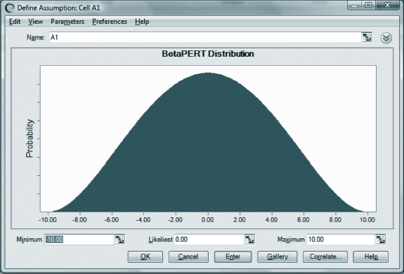
Figure 4-7 Crystal Ball^® dialog box for model inputs assuming the BetaPERT distribution.

When finished with the cash inflow cells, assumption cells for the inflation values in column G need to be defined. For these cells select the Normal distribution. We decided earlier to use a 2 percent inflation rate, plus or minus 1 percent. Recall that the normal distribution is bell-shaped and that the mean of the distribution is its center point. Also recall that the mean, plus or minus three standard deviations, includes 99+ percent of the data. The Normal Distribution dialog box, Figure 4-8, calls for the distribution's mean and its standard deviation. The mean will be 0.02 (2 percent) for all cells. The standard deviation will be .0033 (one-third of the ± percent range). (Note that Figure 4-8 displays only the first two decimal places of the standard deviation. The actual standard deviation of .0033 is used by the program, but if you wish to see the .0033 you may click on “Preferences” at the top of the box. Then click on “Chart,” “Axis,” “Cell format,” “Number,” and change the “2” to “4.” “OK” your way back to the input data sheet.) As you enter these data, the distribution will show a mean of 2 percent and a range from 1 percent to 3 percent.

Figure 4-8 Crystal Ball^® dialog box for model inputs assuming the normal distribution.

Notice that there are two cash outflows for the year 2013, but one of those occurs at the beginning of the year and the other at the end of the year. The entry at the beginning of the year is not discounted, so there is no need for an entry in G4. (Some versions of CB insist on an entry, however, so go ahead and enter 2 percent with zero standard deviation.) Move on to cell G5, in the Name: textbox for the cell G5 enter Inflation Rate. Then enter .02 in the Mean textbox and .0033 in the Std. Dev. textbox. While the rate of inflation could be entered in a similar fashion for the following years, a more efficient approach is to copy the assumption cell G5 to G6. Since CB is an addin to Excel^®, simply using Excel^®'s copy and paste commands will not work. Rather, CB's own copy and paste commands must be used to copy the information contained in both assumption and forecast cells. The following steps are required:

1. Place the cursor on cell G5.
2. Click on “Copy” in the Crystal Ball ribbon.
3. Highlight the range G6:G14.
4. Click on “Paste” in the Crystal Ball ribbon.

Note that 2022 has two cash inflows, both occurring at the end of the year. Because we don't want to generate two different rates of inflation for 2022, the value generated in cell G14 should be used for both 2022 entries. Type =G14 in the G15 cell. Now we consider the forecast or outcome cell. In this example we wish to find the net present value of the cash flows we have estimated. The process of defining a forecast cell involves four steps.

1. Click on the cell F17 to select it as containing an outcome that interests us.
2. Select the menu option Define Forecast from the Crystal Ball ribbon at the top of the screen.
3. CB's Define Forecast dialog box is now displayed. In the Name: textbox, enter a descriptive name such as Net Present Value of Project. Then enter a descriptive label such as Dollars in the Units: textbox.
4. Click OK. There is only one Forecast cell in this example, but in other situations there may be several. Use the same four steps to define each of them.

When you have completed all entries, what was Table 4-5 is now changed and appears as Table 4-7.

We are ready to simulate. CB randomly selects a value for each assumption cell based on the probability distributions which we specified and then calculates the net present value of the cell values selected. By repeating this process many times, we can get a sense of the distribution of possible outcomes, or in this case the distribution of NPVs for this project.

Approximately in the center of the CB ribbon, you will see the Run Preferences. Below it is the “Trials” box. It should be set to “1000.” If not, simply enter 1000 in the box. To run the simulation, click the green Start Arrow in the CB ribbon.

Table 4-7 Three-Point Estimate of Cash Flows and Inflation Rate for PsychoCeramic Sciences, Inc. All Assumption and Forecast Cells Defined

The distribution of NPVs resulting from simulating this project 1,000 times is displayed in Figure 4-9. Statistical information on the distribution is shown in Figure 4-10. The NPVs had a mean of $11,086 and a standard deviation of $8,115. We can use this information to make probabilistic inferences about the NPV of the project such as what is the probability the project will have a positive NPV, what is the probability the project's NPV will exceed $10,000, or what is the probability the project's NPV will be between $5,000 and $10,000?

Figure 4-9 Frequency chart of the simulation output for net present value of Psycho-Ceramic Sciences, Inc. Project.

CB provides considerable information about the forecast cell in addition to the frequency chart including percentile information, summary statistics, a cumulative chart, and a reverse cumulative chart. For example, to see the summary statistics for a forecast cell, click on the Extract Data button in the CB ribbon and check Statistics in the dialog box that is displayed. The Statistics view for the frequency chart (Figure 4-9) is illustrated in Figure 4-10.

Figure 4-10 contains some interesting information. There are, however, several questions that are more easily answered by using Figure 4-9, the distribution of the simulation's outcomes. What is the likelihood that this project will achieve an NPV at least $10,000 above the hurdle rate including inflation? It is easy to answer this question. Note that there are black triangles at either end of the baseline of the distribution in Figure 4-9. By placing the cursor on the triangle on the left end of the simulation distribution baseline and sliding it to the $10,000 mark, the probability of a $10,000 or greater outcome can be read in the “Certainty” box. One can also find the same answer by deleting the “−Infinity” in the box in the lower left corner of the Frequency View and entering $10,000 in it.

Figure 4-10 Summary statistics of the PsychoCeramic Sciences, Inc. simulation.

Even in this simple example, the power of including uncertainty in project budgets should be obvious. Because a manager is always uncertain about the amount of uncertainty, it is also possible to examine various levels of uncertainty quite easily using CB. We could, for instance, alter the degree to which the inflow estimates are uncertain by expanding or contracting the degree to which optimistic and pessimistic estimates vary around the most likely estimate. We could increase or decrease the level of inflation. Simulation runs made with these changes provide us with the ability to examine just how sensitive the outcomes (forecasts) are to possible errors in the input data. This allows us to focus on the important risks and to ignore those that have little effect on our decisions.

Considering Disaster

In our consideration of risk management in the PsychoCeramic Sciences example, we based our analysis on an “expected value” approach to risk. The expected cost of a risk is the estimated cost of the risk if it does occur times the probability that it will occur. How should we consider an event that may have an extraordinarily high cost if it occurs, but has a very low probability of occurring? Examples come readily to mind: the World Trade Center destruction of 9/11, Hurricane Katrina, the BP oil spill in the Gulf of Mexico, the Hurricane Sandy floods of 2012 (a supposedly 500-year event!). The probability of such events occurring is so low that their expected value may be much less than some comparatively minor misfortunes with a far higher probability of happening.

If you are operating a business that uses a “just in time” input inventory system, how do you feel about a major fire at the plant of your sole supplier of a critical input to your product? The supplier reports that their plant has never had a major fire, and has the latest in fire prevention equipment. Does that mean that a major plant fire is impossible? Might some other disaster close the plant—a strike, an al Qaeda bomb? Insurance comes immediately to mind, but getting a monetary pay-back is of little use when you are concerned with the loss of your customer base or the death of your firm.

In an excellent book, The Resilient Enterprise, Yossi Sheffi (Sheffi, 2005) deals with the risk management of many different types of disasters. He details the methods that creative businesses have used to cope with disasters that struck their facilities, supply chains, customers, and threatened the future of their firms. The subject is more complex than we can deal with in these pages, but we strongly recommend the book, a “good read,” to use a reviewer's cliché.

We are now ready to consider the scheduling problem. Because durations, like costs, are uncertain, we will continue our discussion of the matter, adding some powerful but reasonably simple techniques for dealing with the uncertainty surrounding both project schedule and cost.

    REVIEW QUESTIONS

1. Contrast the disadvantages of top-down budgeting and bottom-up budgeting.
2. What is the logic in charging administrative costs based on total time to project completion?
3. Would you expect a task in a manufacturing plant that uses lots of complex equipment to have a learning curve rate closer to 70 percent or 95 percent?
4. How does a tracking signal improve budget estimates?
5. Are there other kinds of changes in a project in addition to the three basic types described in Section 4.4? Might a change be the result of two types at the same time?

    DISCUSSION QUESTIONS

6. Given the tendency of accountants to allocate a project's estimated costs evenly over the duration of the task, what danger might this pose for a project manager who faces the following situation? The major task for a $5 million project is budgeted at $3 million, mostly for highly complex and expensive equipment. The task has a six-month duration, and requires the purchase of the equipment at the beginning of the task to enable the project team to conduct the activities required to complete the task. The task begins December 1.

7. The chapter describes the problems of budgeting projects with S-shaped and J-shaped life-cycle curves. What might be the budget problems if the life cycle of a project was just a straight diagonal line from 0 at project start to 100 percent at project completion?

8. If a firm uses program budgeting for its projects, is an activity budget not needed? If it is, then of what value is the program budget?

9. As a senior manager, you oversee a project with a total estimated cost of 245 engineer-months of effort. Three months ago, however, the project had fallen behind by about 25 engineer-months so you authorized the hiring of three additional engineers, which you felt should more than make up for the delay in the remaining year of the project (3 × 12 months = 36 engineer-months). You have just received the latest quarterly project status report and are surprised to learn that the project is now 40 engineer-months behind schedule! Your first reaction is to calculate how many more engineers need to be hired to make up for the increased delay. Using Brooks's concept of the “mythical man month,” explain what might be happening here.

10. So what was wrong with the purchasing manager's assistant's solution (outlined in Section 4.3) to the problem of having an inadequate supply of hard-to-obtain parts?

11. Contrast simulation to other risk analysis tools discussed in Chapter 3 such as decision tables, FMEA, logic charts, and contingency planning. What are its advantages and disadvantages? If you were to do an important risk analysis, which tool would you prefer?

    PROBLEMS

12. Your firm designs PowerPoint slides for computer training classes, and you have just received a request to bid on a contract to produce the slides for an 8-session class. From previous experience, you know that your firm follows an 85 percent learning rate. For this contract it appears the effort will be substantial, running 50 hours for the first session. Your firm bills at the rate of $100/hour and the overhead is expected to run a fixed $600 per session. The customer will pay you a flat fixed rate per session. If your nominal profit margin is 20 percent, what will be the total bid price, the per session price, and at what session will you break even?

13. In the template for finding bias (Fig. 4.3), using the Actuals as shown, compare the estimating model shown in the figure with the following estimates:

Base your comparison on the mean bias and the MAR. Comment.

14. The IT unit of a company has been asked to prepare a budget for a special software package project. The group has considerable experience with similar tasks and submits the costs in the following table. The group also thinks that the distribution of the hours worked for each phase is normal. The wage rate for the software engineers employed on each phase is $60 per hour. Using simulation, find the distribution of total engineering costs for all the phases. What is the average engineering cost? Also, find the probability that the total engineering cost will be less than $85,000.

15. Reconsider the following problem from Chapter 1: A 4-year financial project is forecast to have net cash inflows of $20,000; $25,000; $30,000; and $50,000 in the next 4 years. It will cost $75,000 to implement the project, payable at the beginning of the project. If the required rate of return is 0.2, conduct a discounted cash flow calculation to determine the NPV. Now, however, assume that the net cash inflows are probabilistic variables. Further assume that each forecast net cash inflow is normally distributed with standard deviations of $1,000, $1,500, $2,000, and $3,500, respectively. Given a required rate of return of 0.2, find the mean forecast NPV using Crystal Ball^®. What is the probability that the actual NPV will be positive?

16. What would happen to the NPV of the above project if the inflation rate was expected to be 4 percent in each of the next 4 years? You may use either Excel^® or Crystal Ball^® to determine your answer.

17. Information about the cash flows for a 4-year financial project is listed in the following table. The cash flows are assumed to follow a triangular distribution. The cost of implementing the project is expected to be between $60,000 and $70,000, with all values in this range being equally likely. Analysis of changes in the Consumer Price Index suggests that the annual rate of inflation can be approximated with a normal distribution with a mean of 4 percent and standard deviation of 1.5 percent. The organization's required rate of return is 20 percent. Develop a model in Crystal Ball^® to analyze this situation and answer the following questions.

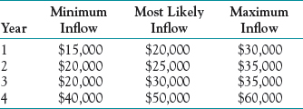
(a) What is the expected NPV of this project?

(b) What is the range of NPVs?

(c) How would you characterize the level of risk associated with this project?

(d) Would you recommend undertaking the project? Why or why not?

18. Server Farm Inc. (SFI) needs to upgrade its server computers. Company management has identified the following two options: (1) shift to a Windows-based platform from its current Unix-based platform, or (2) stick with a Unix-based platform. It is standard practice at SFI to use a triangular distribution to model uncertain costs.

Along these lines, the company estimates that if it migrates to Windows, the new server hardware could cost as little as $100,000 or as much as $200,000. The technical group's best estimate is that the hardware costs will be $125,000 if the Window's option is pursued. Likewise, the company's best guess regarding the cost to upgrade and convert its software to Windows is $300,000 with a range of $275,000 to $500,000. Finally, if the company converts to Windows, employee training costs are estimated to range between $9,000 and $15,000, with the best guess being $10,000. If the company sticks with Unix, the new server hardware will most likely cost $100,000, but could cost as little as $80,000 or as much as $210,000. Software conversion and upgrade costs are expected to be $300,000 but could be as low as $250,000 and as high as $525,000. Employee training costs should fall between $8,000 and $17,500, with a best guess of $10,000. Develop a model to simulate this situation using Crystal Ball^® and answer the following questions.

(a) What is the expected cost of each project?

(b) What is the probability that each project's cost will exceed $575,000?

(c) Which project would you consider to be the most risky?

(d) Which project would you recommend SFI undertake? Why?

19. A light manufacturing firm has set up a project for developing a new machine for one of its production lines. The most likely estimated cost of the project itself is $1,000,000, but the most optimistic estimate is $900,000 while the pessimists predict a project cost of $1,200,000. The real problem is that even if the project costs are within those limits, if the project itself plus its implementation costs exceed $1,425,000, the project will not meet the firm's NPV hurdle. There are four cost categories involved in adding the prospective new machine to the production line: (1) engineering labor cost, (2) nonengineering labor cost, (3) assorted material cost, and (4) production line down-time cost.

The engineering labor requirement has been estimated to be 600 hours, plus or minus 15 percent at a cost of $80 per hour. The nonengineering labor requirement is estimated to be 1500 hours, but could be as low as 1200 hours or as high as 2200 hours at a cost of $35 per hour. Assorted material may run as high as $155,000 or as low as $100,000, but is most likely to be about $135,000. The best guess of time lost on the production line is 110 hours, possibly as low as 105 hours and as high as 120 hours. The line contributes about $500 per hour to the firm's profit and overhead. What is the probability that the new machine project will meet the firm's NPV hurdle?

    INCIDENTS FOR DISCUSSION

A Budgeting Novice

Alexander Jones was an experienced project manager of a small machine shop. He had always had complete authority when working with the clients on specifications of the projects as well as when working with the project team on the schedule. His boss, however, did not feel comfortable letting Alex determine project budgets. The boss always did that himself.

A client approached Alex about designing a piece of surgical equipment. Alex was excited about this project because his usual job was to design and make parts of factory equipment. He was delighted to have a chance to do something that might directly affect humankind. Alex knew what the surgical tool was intended to do and had figured out what had to be done to design and manufacture it. He had even estimated the labor-hour requirement. He wanted to do all the planning discussions with the client, including discussions on the budget.

Questions: What do you think Alex should show to his boss so that the boss would feel more comfortable letting Alex determine and monitor the project's budget? What should Alex say to persuade the boss?

Stealth Electronics

Stealth Electronics manufactures secret electronic weapon systems. They have just engineered a new system. They bid for and won a contract with DARPA (Defense Advanced Research Projects Agency). Stealth Electronics negotiated a cost plus contract for development of the prototype. The prototype project was approximately on time and on budget. They are about to submit a bid to produce the first 25 electronic weapon systems. The production contract will be a fixed fee. The CFO of Stealth Electronics has examined the costs associated with building the prototype and thinks the proposed bid for production of the first 25 systems is significantly too low.

Question: What should the CFO do?

General Sensor Company

Justin Jordan has been named Project Manager of the General Sensor Company's new sensor manufacturing process project. Sensors are extremely price sensitive. General has done a great deal of quantitative work to be able to accurately forecast changes in sales volume relative to changes in pricing.

The company president, Guy General, has faith in the sensitivity model that the company uses. He insists that all projects affecting the manufacturing costs of sensors be run against the sensitivity model to generate data to calculate the return on investment. The net result is that project managers, like Justin, are under a great deal of pressure to submit realistic budgets so go/no-go project decisions can be made quickly. Guy has canceled several projects that appeared marginal during their feasibility stages and recently fired a project manager for overestimating project costs on a new model sensor. The project was killed early in the design stages, and 6 months later a competitor introduced a similar sensor that proved to be highly successful.

Justin's dilemma is how to construct a budget that accurately reflects the costs of the proposed new process. Justin is an experienced executive and feels comfortable with his ability in estimating costs of projects. However, the recent firing of his colleague has made him a little gun-shy. Only one stage of the four-stage sensor manufacturing process is being changed. Justin has detailed cost information about the majority of the process. Unfortunately the costs and tasks involved in the new modified process stage are unclear at this point. Justin also believes that the new modifications will cause some minor changes in the other three stages, but these potential changes have not yet been clearly identified. The stage being addressed by the project represents almost 50 percent of the manufacturing cost.

Questions: Under these circumstances, would Justin be wise to pursue a top-down or a bottom-up budgeting approach? Why? What factors are most relevant here?

St. Dismas Assisted Living Facility Project Budget Development—2

Fred Splient gave his ALF Project Steering Committee 2 months to develop an action plan for their area of responsibility in the project. Each member was told to include the tasks, predecessors and successors, resources needed, responsible person, and an estimated cost. He asked that these be presented to the steering team on August 31.

All through July the ALF project team scrambled to identify the steps required to open the facility and to determine what it would cost. Each team member met with his or her departmental staff to get help in identifying what was needed. For example, the COO spoke with the Dietary Department head and asked that she develop a plan to meet all requirements to set up the facility to feed the residents. The COO then asked the Facilities Manager to develop an action plan to prepare the building and maintain it. The COO also met with the Rehab Services Medical Director and his clinical staff to identify the residents' probable medical needs based on the projected population, and to develop an action plan to prepare to meet the residents' health needs. The COO asked the therapy manager to prepare a plan to develop social activities for the residents.

Everyone on the team called the Chief Financial Officer for help in determining the budgets for their action plans. The CFO also had to validate the estimates of cost and revenue from facility operations, and to project earnings and return on the investment. Like any good administrator, when the CFO realized he had no expertise in this area, he hired a consultant to help him determine the project costs and budget. Dr. Sara Sharf was chosen as the consultant—she had over 5 years' experience in developing business plans for assisted living facilities.

Dr. Sharf recommended that St. Dismas target the middle income geriatric population since there were many up-scale facilities in the area. Dr. Sharf and the market researchers determined what level of rent people in that population could and would pay. They then looked at what needed to be in the facility to meet the needs of their targeted population. After additional site visits of facilities and meetings with the selected construction contractor, they finalized the layout of units and common space areas that would be included in the design. The Construction Project Manager requested and received an action plan and cost estimate from the construction contractor. The contractor had estimated that construction cost would probably run about $70 per square foot with a standard deviation of $3.67. He could not be absolutely sure because of potential change orders. He emphasized that the estimates assumed that the project would be completed without further changes in its design concept.

While the CFO was haggling with the construction contractor about determining a more accurate cost estimate, he received a phone call from Dr. Zen Link, the Head of Geriatric Medicine at St. Dismas. Dr. Link's secretary had seen men measuring the land behind the parking lot and she wanted to know what was going on; so did Dr. Link. Since Dr. Link was one of the hospital's best referrers, the CFO told him about the potential project. Dr. Link felt that his input was needed up front as he was the only person on staff who would know the health needs of the facility's residents and appropriate equipment needs and staffing models that should be set up. With Dr. Link's input, the CFO estimated the operating costs to run the facility and projected the occupancy rates needed to cover those costs. The Rehab Services Medical Director, who was a member of the original project team, was quite upset when he saw Dr. Link's budget for the medical equipment that was to be purchased for the facility. The Medical Director felt that Dr. Link wanted to purchase too much expensive equipment, which was not necessary to have on site. The hospital had the majority of the equipment that was necessary and there was no need to duplicate it, thus inflating that portion of the budget. The CFO did not want to get in the middle of their argument so he left Link's budget just as Link submitted it and hoped someone would raise the issue at the next Steering Team Meeting. The CFO was quite concerned about the lack of experience of the team in developing such a budget, and he felt that there was far more uncertainty in the budget than the estimates reflected.

With the construction cost estimate and an outline of the services to be provided, the following projected capital expenditure was developed.

The CFO developed an income statement for the next 20 years. The first 3 years are shown below.

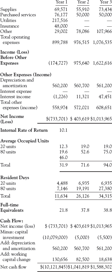
The CFO, Dr. Sharf, and the Projct Steering Team were ready to combine their individual plans and costs into a composite plan and budget.

    QUESTIONS

1. The cost per square foot for the units is given in the text together with its standard deviation. What other areas of cost or revenue are likely to have cost uncertainty? How should these uncertainties be handled?
2. How would you suggest the team handle the issue of Dr. Link's supposedly inflated medical equipment costs?

Photstat Inc.

Photstat Inc. is contemplating the formation of a project team to develop a new service. Briefly, the service would allow customers to order customized mouse pads over the Internet based on photographs or other artwork sent electronically to the firm.

The company estimates that the price of the mouse pad will be between $10 and $15 per unit, with all prices in this range equally likely. Based on historical data, Photstat estimates that the total market size for these types of products in their first year follows a normal distribution with a mean of 100,000 units and a standard deviation of 10,000. Again, according to historical data, Photstat's market share tends to be normally distributed with a mean of 30 percent and standard deviation of 3 percent. Market growth tends to follow a normal distribution growing an average of 10 percent per year with a standard deviation of 3 percent. Estimates from the equipment manufacturer selected to design and produce the required equipment indicate that the cost of the equipment is normally distributed with a mean of $500,000 and a standard deviation of 60,000. Historical data indicate there is a 10 percent chance that the equipment will last for only 3 years. Similarly, there is a 60 percent chance the equipment will last 6 years, a 20 percent chance it will last 8 years, and a 10 percent chance the equipment will last 10 years. The variable costs of similar products were found to be normally distributed with a mean of $3 and a standard deviation of $0.25. Finally, an economic analysis undertaken by the firm suggests that the rate of inflation in any given year is normally distributed with a mean of 3 percent and a standard deviation of 0.5 percent.

    QUESTIONS

1. What is the expected value of the project?
2. Simulate this project 1000 times and compute the average profit over the 1000 replications. Plot a histogram of the outcomes of the 1000 replications.
3. How does the average of the simulation compare to the expected value you calculated? What are the managerial implications of this difference?

Building the Geddy's dream house

Neil and Alexis Geddy graduated from college 5 years ago. Since graduating, Neil has been working as an engineer while Alexis has been working in marketing. Initially, the young couple focused on paying off their student loans which they were able do in a little more than 2 years. Since paying off their student loans, the couple have been diligently saving for the downpayment on a house which they would like to build. Neil and Alexis feel they currently have ample savings for the downpayment and are excited to start building their dream house.

Based on their current incomes and the amount they have saved for the down payment, Neil and Alexis would like to spend no more than $350,000 on the construction of their house, but believe they could swing spending as much as $375,000. For the past couple of months the couple have been talking to people they know who have built houses, researching homebuilding websites, and visiting building supply stores to better understand the costs and process associated with building a custom home. Table A summarizes the couple's cost estimates based on what they have learned.

As shown in the table, Neil and Alexis developed three cost estimates for each expense category. The most likely estimate corresponds to the option they would choose (e.g., doors, cabinets) or what the expected costs of an activity would be baring unforeseen difficulties. The pessimistic cost estimates represent the cost if they decided to splurge or if particular challenges were encountered. Finally, the optimistic costs represent opportunities for them to go with lower cost options or in cases where the progress on the activity goes better than expected.

Table A Construction Cost Estimates

    QUESTIONS

1. Based on only the couple's most likely cost estimates, what would you estimate the cost of building the house to be? How does this value compare to what the Geddys budgeted?
2. Simulate this project 10,000 times assuming the expenses follow a triangular distribution. Based on simulation analysis, what is the expected cost of building the house? How does the expected value from the simulation compare to your answer in the previous question? How do you reconcile any differences between the two? Which estimate do you have more confidence in?
3. What are the maximum and minimum amounts the couple can expect to spend on the house?
4. What is the probability that constructing the house will exceed $350,000? What is the probability the costs will be less $375,000? What is the probability that constructing the house will cost between $350,000 and $375,000? Based on your analysis how concerned should the couple be?
5. Assume that 2 months into the construction of the house, the couple decide they need the services of an interior designer to help them with making the right choices. After making a few calls, the couple estimate that, most likely, hiring an interior designer will cost $2,500. However, if they use the interior designer minimally, they could reduce the cost to $1,500 while if they need to rely on the interior designer more than they expect, the cost could reach $5,000. Modify your simulation model to incorporate the cost of an interior designer. What impact does this change have on the construction budget?

    BIBLIOGRAPHY

ABRAMS, S. “The Big Dig,” Kennedy School Bulletin, Harvard University, Cambridge, MA Spring 2003.

AMOR, J. P., and C. J. TEPLITZ. “An Efficient Approximation for Project Composite Learning Curves.” Project Management Journal, September 1998.

BADIRU, A. B. “Incorporating Learning Curve Effects into Critical Resource Diagramming.” Project Management Journal, June 1995.

BREYFOGLE, F. W., III. Implementing Six Sigma: Smarter Solutions Using Statistical Methods. 2nd ed., Hoboken: John Wiley, 2003.

BROOKS, F. P. The Mythical Man-Month. Reading, MA: Addison-Wesley, 1975.

CAMM, J. D., J. R. EVANS, and N. K. WOMER. “The Unit Learning Curve Approximation of Total Cost.” Computers in Industrial Engineering. Vol. 12, No. 3, 1987.

EVANS, J. R., and D. L. OLSON. Introduction to Simulation and Risk Analysis. Upper Saddle River, NJ: Prentice Hall, 1998. (An excellent book using Crystal Ball^® software.)

GAGNON, R. J., and S. J. MANTEL, Jr. “Strategies and Performance Improvement for Computer-Assisted Design.” IEEE Transactions on Engineering Management, November 1987.

HAMBURGER, D. H. “Three Perceptions of Project Cost—Cost Is More Than a Four Letter Word.” Project Management Journal, June 1986. (Recommended reading for any project manager who is not familiar with accounting.)

HERTZ, D. B., and H. THOMAS. Risk Analysis and Its Applications. New York: Wiley, 1983. (The name “Hertz” is almost synonymous with risk analysis, particularly strong in the area of financial risk.)

LAWRENCE, A. O. “Using Automated Estimating Tools to Improve Project Estimating.” PM Network, December 1994.

LIBERATORE, M. J., and G. J. TITUS. “The Practice of Management Science in R & D Project Management.” Management Science, August 1983.

MALLAK, L. M., H. A. KURSTEDT, Jr., and G. A. PATZAK. “Planning for Crises in Project Management.” Project Management Journal, June 1997.

MARTIN, J. E. “Selecting an Automated Estimating Tool for IS Development Projects.” PM Network, December 1994.

MCCARTHY, J. Dynamics of Software Development. Redmond, WA: Microsoft Press, 1995. (An excellent read-and-enjoy book that is not just for software projects. It is packed with irreverent good sense.)

MEREDITH, J. R. and S. M. SHAFER. Operations Management for MBAs. Hoboken, NJ: Wiley, 2003.

PMI. “Digging Deep,” PM Network, August 2004.

PMI. “Polluted Progress,” PM Network, March 2005.

PMI Standards Committee. A Guide to the Project Management Body of Knowledge, 5th ed. Newtown Square, PA: Project Management Institute, 2013.

PYZDEK, T. The Six Sigmas Handbook, Revised and Expanded: The Complete Guide for Greenbelts, Blackbelts, and Managers at All Levels. New York: McGraw Hill, 2003.

Rath & Strong's Six Sigma Pocket Guide. Rath & Strong Management Consultants, Lexington, MA: 2000.

SIMON, H. The New Science of Management Decisions, rev. ed. Englewood Cliffs, NJ: Prentice Hall, 1997. (An excellent and readable classic on management science with a particularly good introduction to risk analysis.)

SWANSON, S. A. “Estimating Errors,” PM Network, October 2011.

WHEATLEY, M. “Making the Cut.” PM Network, June 2009.