Scheduling the Project

Consider the job of planning a project, developing a budget for it, and scheduling all of the many tasks involved. It should be obvious that these three activities are not actually separable. Because a budget must include both the amounts and timing of resources received or expended, one cannot prepare a budget without knowing the specifics of each task and the time period(s) during which the task must be undertaken. Similarly, the project plan implies a schedule just as a schedule implies a plan. It is useful to begin study of these interdependent, partial descriptions of a project with an examination of the planning process because this process is the foundation of all that follows. The decision about whether to turn our attention first to the budget or the schedule is arbitrary. We chose the budget largely because most readers have some familiarity with the subject. The problem is that planning, budgeting, and scheduling are parts of the same basic process. They are considered separately only because we cannot write about all three at the same time.

The project schedule is simply the project plan in an altered format. It is a convenient form for monitoring and controlling project activities. Actually, the schedule itself can be prepared in several formats. PMBOK covers some of these in Chapter 6 on Project Time Management. In this chapter, we describe the most common formats—Gantt charts and PERT/CPM networks—and demonstrate how to convert a project plan or WBS into these formats. We also note some of the strengths and weaknesses of the different displays. In addition, we apply risk management directly to the project schedule. From this analysis we show how to estimate the likelihood that a project can be completed on or before a specific time. (In Chapter 6, we explore what to do if it appears that the project will not be completed on schedule.) In addition to standard analytic methods for risk management, we once again demonstrate simulation methods.

We start with simple plans and schedule them manually. After scheduling by hand, we turn to the computer and use MSP to do our scheduling and many other tasks for us. The same approach is used for risk management. First, problems involving risk will be solved by hand. Once the theory is understood, we use the computer to handle the same problems without so much arithmetic.

5.1 PERT AND CPM NETWORKS

In the late 1950s, the Program Evaluation and Review Technique (PERT) and the Critical Path Method (CPM) were independently developed. PERT was developed by the U.S. Navy, Booz-Allen Hamilton (a business consulting firm), and Lockheed Aircraft (now Lockheed Martin Corp.); and CPM was developed by Dupont De Nemours Inc. When they were developed, there were significant differences in the methods. For example, PERT used probabilistic (or uncertain) estimates of activity durations and CPM used deterministic (or certain) estimates but included both time and cost estimates to allow time/cost trade-offs to be used. Both methods employed networks to schedule and display task sequences. (Throughout this chapter, we will use the words “activity” and “task” as synonyms to avoid constant repetition of one or the other.) Both methods identified a critical path of tasks that could not be delayed without delaying the project. Both methods identified activities with slack (or float) that could be somewhat delayed without extending the time required to complete the project. While PERT and CPM used slightly different ways of drawing the network of activities, anything one could do with PERT, one could also do with CPM and vice versa. When writing about the history of project management, differentiating PERT and CPM is important and interesting. When managing projects, the distinction is merely fussy. Traditional PERT is used less often than CPM; but CPM can be used with three-time estimates, and we can do things with PERT that were restricted to CPM in “olden times.” We use both names because users in the real world are apt to use either.

The Language of PERT/CPM

Several terms used in discussing PERT/CPM analysis have been adopted from everyday language but have quite different meanings than in common usage. These terms are defined here as used in PERT/CPM.

Activity—A task or set of tasks required by the project. Activities use resources and time.

Event—An identifiable state resulting from the completion of one or more activities. Events consume no resources or time. Before an event can be achieved or realized, all its predecessor activities must be completed.

Milestones—Identifiable and noteworthy events marking significant progress on the project.

Network—A diagram of nodes (may represent activities or events) connected by directional arcs (may represent activities or simply show technological dependence) that defines the project and illustrates the technological relationships of all activities. Networks are usually drawn with a “Start” node on the left and a “Finish” node on the right. Arcs are always tipped with an arrowhead to show the direction of precedence, that is, from predecessors to successors.

Path—A series of connected activities (or intermediate events) between any two events in a network.

Critical path—The set of activities on a path from the project's start event to its finish event that, if delayed, will delay the completion date of the project.

Critical time—The time required to complete all activities on the critical path.

In Chapter 3, on planning, we noted that tasks may be divided into subtasks and each of the subtasks may be further divided. To carry out this process, it is necessary to know which tasks are immediate predecessors or successors of which others. The predecessor/successor relationship defines technological dependence. (See Chapter 3, Section 3.3.)

Building the Network

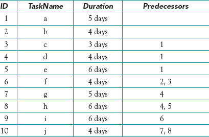
There are two ways of displaying a project network. In one we depict the activities as arrows and events as nodes. This gives an activity-on-arrow (AOA) network, usually associated with PERT. Alternatively, we can create an activity-on-node (AON) network by showing each task as a node and linking the nodes with arrows that show their technological relationship. The AON network is often associated with CPM. To understand the distinction, let us assume a small project represented by the tasks and precedences shown in Table 5-1.

Because it is easiest to draw, we start with the AON network. Because tasks a and b have no predecessors, they follow the Start node. We connect them to the starting node with arrows as in Figure 5-1.

Note that task c has a as a predecessor and that tasks d and e have b as their common predecessor as shown in Figure 5-2.

The network is easily completed. Task f has both c and d as predecessors, while g follows e. Because there are no more tasks, we can tie all loose ends to a node labeled Finish as in Figure 5-3.

The AOA network is generally more difficult to draw, but depicts the technical relationships of the activities quite well. Beginning the same way, we create a Start node from which flow all activities that have no predecessors, in this case a and b. The completion of these activities results in events (nodes, often drawn as circles) numbered 1 and 2 for easy identification as in Figure 5-4.

Table 5-1 A Sample Set of Project Activities and Precedences

Task	Predecessor
a	—
b	—
c	a
d	b
e	b
f	c, d
g	e

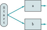
Figure 5-1 Stage 1 of a sample AON network from Table 5-1.

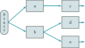
Figure 5-2 Stage 2 of a sample AON network from Table 5-1.

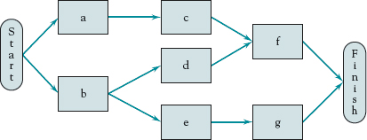
Figure 5-3 A completed sample AON network from Table 5-1.

Figure 5-4 Stage 1 of sample AOA network from Table 5-1.

Figure 5-5 Stage 2 of a sample AOA network from Table 5-1.

Table 5-1 indicates that task a precedes task c, and that task b precedes both tasks d and e. Figure 5-5 shows these additions with event nodes 3, 4, and 5, as indicated.

We are left with two activities, f and g. Task f has two predecessors, c and d. This means that tasks c and d actually finish at the same node (or event) and that f cannot start until this event is achieved, that is, until both c and d are completed. Task g is preceded by e. Table 5-1 shows no more tasks, and as in the case of the AON network this means that all tasks with no successors should go to a node labeled Finish. See Figure 5-6(a) in which the nodes have been renumbered and some combined for viewing simplicity.

We can handle f in a simpler though equivalent way by connecting the nodes following c and d in Figure 5-5 with an arrow drawn with a dashed line, see Figure 5-6(b). This is called a dummy activity and merely shows a technological linkage. Generally speaking, dummy tasks are used in situations where two activities have the same starting and finishing nodes or where a single activity connects to two or more nodes. The problem with two activities sharing the same starting and finishing nodes is that it becomes difficult to distinguish the tasks from one another. One solution to this problem is to add an extra ending node for one of the tasks and then draw a dummy task from the new node to the previously shared node. Adding a dummy task in this situation ensures that the tasks have unique identities while at the same time maintaining the correct technological precedence relationships. Dummy tasks require no time and no resources.

With occasional exceptions for clarity, we will use AON networks throughout this book because they are used by most of the popular project management software. An important advantage of AON notation is that the networks are easy to draw. AOA networks, particularly when they have more than 15 or 20 activities, are difficult to draw by hand. With modern software this is not a serious problem, but the software that generates AOA networks is quite expensive. AON networks often do not show events, but it is simple enough to add them by showing the event (usually a milestone) exactly as if it were an activity but with zero time duration and no resources. The PM should be familiar with both types of networks.

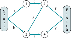
Figure 5-6(a) A completed sample AOA network from Table 5-1.

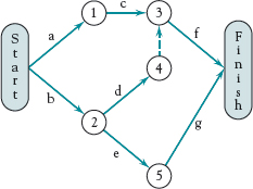
Figure 5-6(b) A completed sample AOA network showing the use of a dummy task, Table 5-1.

Table 5-2 A Sample Problem for Finding the Critical Path and Critical Time

Finding the Critical Path and Critical Time

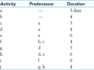
Let us now consider a more complicated example. Given the data in Table 5-2, we can start drawing the associated AON network as in Figure 5-7. The activity names and durations are shown in the appropriate nodes.

Note that activity f follows both b and c. If we redraw Figure 5-7 and place the c node below the d and e nodes, we will avoid having several of the arrows crossing one another; see Figure 5-8 for the complete network. This kind of rearrangement is quite common when drawing networks, and most software will allow the user to click and drag nodes around to avoid the confusion of too many crossing arrows.

We can add information to the nodes in the network. Just above each node it is common practice to show what is called the earliest start time (ES) and earliest finish time (EF) for the associated activity. Just below each node is shown the latest start time (LS) and latest finish time (LF) for the activity. The node would appear as in Figure 5-9. The corresponding information for Figure 5-8 is shown in Figure 5-10 and its derivation is described in detail just below.

Activities a and b may start on Day 0, their ESs. Their EFs will be equal to their durations, 5 and 4 days, respectively. Tasks c, d, and e cannot start before a is completed on Day 5. Adding their respective durations to their ESs gives us their EFs, c finishing on Day 8, d on Day 9, and e on Day 11. Task f cannot start before both b and c are finished on Day 8, resulting in the EF for f on Day 12. Similarly, we find EFs for tasks g (9 + 5 = 14) and h (11 + 6 = 17). Recall that a successor cannot be started until all predecessors are completed. Thus, h cannot start until Day 11 when both d and e are finished—Days 9 and 11, respectively. The same situation is true for task j. It cannot be started until both g and h are completed on Day 17, giving an EF of 17 + 4 = 21. Task i, following f, has an EF of 12 + 6 = 18. No tasks follow i and j, completed on Days 18 and 21, respectively. When they are both finished, the project is finished. That event occurs on Day 21.

Figure 5-7 Stage 1 of a sample network from Table 5-2.

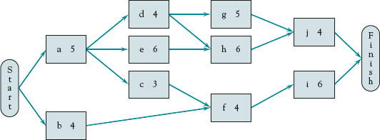
Figure 5-8 A complete network from Table 5-2.

Figure 5-9 Information contents in an AON node.

Figure 5-10 The critical path and time for sample project in Table 5-2.

All activities, and thus all paths, must be completed to finish the project. The shortest time for completion of the network is equal to the longest path through the network, in this case a-e-h-j. If any activity on the a-e-h-j path is even slightly delayed, the project will be delayed and that identifies a-e-h-j as the critical path and 21 days as the critical time. In Figure 5-10 the critical path is depicted by a bold line—a common practice with PERT/CPM networks. We found the ES and EF for each activity quite easily by beginning at the start node and moving from left to right through the network, calculating as we go from node to node. This is called a “forward pass” (or “left-to-right pass”) and makes it simple to find the critical path and time for PERT/CPM networks.

In a similar fashion, we can perform a “backward pass” (or “right-to-left pass”) to calculate the LS and LF values for each activity. Referring to Figure 5-10, we begin by assuming that we would like to complete the project within the critical time identified in the forward pass, 21 days in our example. Clearly, activities i and j must be completed no later than Day 21 in order not to delay the entire project. Therefore, these activities both have LFs of 21.

Given a task time of 4 days, j must be started no later than Day 17 in order to be completed by Day 21. Likewise, task i can be started as late as Day 15 and still finished by Day 21 given its 6-day task time. Because task j cannot be started any later than Day 17, tasks g and h must be completed by Day 17. In a similar fashion, task f must be completed by Day 15 so as not to delay task i beyond its LS. Subtracting the task times from the LF for each of the tasks yields LSs of 11, 11, and 12 for tasks f, h, and g, respectively.

Now consider task d. Task d precedes both tasks g (LS = 12) and h (LS = 11). The question is, should d's LF be 11 or 12? The correct answer is 11. The reason being, if task d were completed on Day 12, task h could not start on its LS of Day 11. Therefore we note that in situations where a particular activity precedes more than one task, its LF is equal to the minimum LSs of all activities it precedes.

The LFs and LSs for tasks b, c, and e are easily calculated since each of these tasks precedes a single task. Task a precedes tasks c, d, and e. Because task e has the lowest LS of 5 days, the LF for task a is calculated to be 5 days.

Calculating Activity Slack

If activities on the critical path cannot be delayed without causing the entire project to be delayed, does it follow that activities not on the critical path can be delayed without delaying the project? As a matter of fact, it does—within limits. The amount of time a noncritical task can be delayed without delaying the project is called slack or float. The slack for any activity is easily calculated as LS — ES = LF — EF = slack.

It should be clear that for any task on the critical path, its LF must be the same as its EF. It therefore has zero slack. If it finishes later than its EF, the activity will be late, causing a delay in the project. (Of course, the statement is equally true for its LS and ES.) This rule holds for activities a, e, h, and j, all on the critical path. But for activities not on the critical path the LF and EF (or the LS and ES) will differ and this difference is the activity slack. Take activity i, for example. It could be completed as early as Day 18 because its ES is Day 12 and it has a 6-day duration. It must, however, be completed by Day 21 or the project will be delayed. Because i has a duration of 6 days, it cannot be started later than Day 15 (21 — 6). Given an LS of 15 and an ES of 12, task i could be delayed up to 3 days (LS — ES or LF — EF) without affecting project completion time. Thus, activity i has 3 days of slack.

For another example, consider task g. It is a predecessor to task j that is on the critical path. Task j must start on Day 17, which gives task g an LF of 17. It has an EF of Day 14 and thus has 3 days of slack.

Now consider a more complex situation: task d. First, task d must be completed by Day 12 so as not to make g late and thus j late and thereby the whole project late! Thus, along this path task d has 3 days of slack in the role as a predecessor of task g. But d is also a predecessor of critical activity h, and along this path task d must be completed by Day 11 or h will be late to start. Task d, therefore, has only 2 days of slack, not 3.

Slack for other tasks are determined in the same way. Task f precedes i, and the latter has an LS of Day 15. Given an LF of 15, f must start no later than Day 11. Its ES of Day 8 means that f has 3 days of slack. Task c is a predecessor of f, and because the latter's LS is Day 11, c must be completed by then. With an LF of 11 and an EF of 8, c has 3 days of slack. The only remaining task to be considered is b. This task is linked to f and, like c, must be complete by f's LS, Day 11. With an EF of Day 4, b has 7 days of slack.

Throughout this discussion of calculating slack, we have made two assumptions that are standard in these analyses. First, when calculating slack for a set of activities on a noncritical path, the calculation for any given activity assumes that no other activity on the path will use any of the slack. Once a project is underway, if a predecessor activity uses some of its slack, its EF is adjusted accordingly and the ESs of successor activities must also be corrected. We have also assumed that the critical time for the project is also the project's due date, but it is not uncommon for a project to have “project slack” (or “network slack”). Our 21-day project might be started 23 days before its promised delivery date, in which case activities on the “critical path” would have 2 days of slack and noncritical activities would have an additional 2 days of slack.

Milestones may be added to the display quite easily: Add the desired milestone event as a node with zero duration. Its ES will equal its EF, and its LS and LF will be equal. Milestones should, of course, be immediate successors of the activities that result in the milestone events. Finally, if a starting date has been selected for the project, it is common to show ES, EF, LS, and LF as actual dates.

Before continuing, a pause is in order to consider the managerial implications of the critical path and slack. The PM's primary attention must be paid to activities on the critical path. If anything delays one of these activities, the project will be late. At the start of the project, the PM correctly notes that activity a is on the critical path and b is not. This raises an interesting question. Can any resources reserved for use on b be borrowed for a few days to work on a and thereby shorten its duration? The nature of b's resources and a's technology will dictate whether or not this is possible. If a, for example, could be shortened a day by using b's resources for 4 days, the critical path would be shortened by a day. This would cause no problem for b, which had 7 days of slack. If the delivery date for the project remains the same, the entire project would then have a day of slack. The presence of project slack tends to lower the PM's pulse rate and blood pressure.

Doing It the Easy Way—Microsoft Project (MSP)

As promised, once the reader understands how to build a network by hand, we can introduce tools provided through project management software. The first task is transferring information from the project plan into the software, MSP in this case. This is not difficult. MSP presents a tab entry table much like the project plan template shown in Table 5-3. It has spaces where the tasks can be identified, plus spaces for activity durations and predecessors. The software automatically numbers each activity that is entered. MSP offers a great number of options for viewing the data once it is entered into the project plan or entry view. If a specific start date or finish date is already determined for an activity, MSP allows you to enter it as well.

Once the project plan data are entered, MSP will automatically draw an AON PERT/CPM network as shown in Figure 5-11. Note that the figure lacks start and finish nodes because they were not entered on the activity list. Note also that the tasks in the network appear with ID numbers in order, flowing from left to right and from the top to the bottom. In Figure 5-11 several arrows cross, which may be confusing. The nodes show the activity name, ID number, duration, and start and finish times. These nodes are easily customized to show many different things concerning each specific activity.

Table 5-3 An MSP Version of Sample Problem in Table 5-2

It is simple to add Start and Finish nodes as milestones to make the network easier to understand. An activity named “Start” is entered at the top of the list, and an activity named “Finish” at the bottom. We want these activities to appear as milestones, significant events in the life of the project. In MSP a milestone is an activity with a duration of 0. Because we want the Start and Finish milestones to be linked to the beginning and ending activities of the project, all predecessors will have to be changed in light of these additions. For example, a and b will now have Start as a predecessor, and the last two activities, i and j, are predecessors to Finish. (In MSP, predecessors are indicated by task ID numbers rather than the task names used here for clarity.)

Figure 5-11 An MSP version of PERT/CPM network from Table 5-3.

Figure 5-12 A modified version of MSP network from Figure 5-11.

Redrawing the network to get rid of the crossing arrows is also simple. As we noted when drawing the network manually, this is corrected by moving the c, f, and i nodes down to the bottom of the network. In MSP, that is easily done by simply dragging the nodes to whatever location you wish. See Figure 5-12 for the results of both changes. Notice in Figure 5-12 that because we added Start and Finish to the activity list, the other activities have been renumbered to conform to the changed list.

MSP will also calculate slack. (For details, click on MSP's “Help,” type “Slack,” and follow the directions.) MSP, and some writers, differentiate between “total slack” and “free slack.” Total slack is LF — EF or LS — ES as we explained in the section just above. Free slack is defined as the time an activity can be delayed without affecting the start time of any successor activity. Take activity b for example. Its EF is 4 days, but it could be finished as late as 8 days without affecting task f in any way. It is thus said to have 4 days of free slack. Using b as an example, the rule for calculating free slack for an activity is

The total slack for b is seven days, as we calculated in the section on finding slack.

These same calculations can be done by using the Solver in Excel^®. To see how this is accomplished, refer to Lawrence and Pasternak (1998, Chapters 5 and 6). Finding the critical path is a fairly straightforward problem in linear programming, but it often takes more time than doing the same problem by hand, and certainly much more time (entering the required information) than letting MSP solve the problem.

5.2 PROJECT UNCERTAINTY AND RISK MANAGEMENT

In Chapter 4, Section 4.5 on risk analysis mentioned making most likely (or normal), optimistic, and pessimistic cost estimates for project tasks. Such estimates were shown in Table 4-6, and we promised to illustrate how to use these and similar estimates of task duration to determine the likelihood that a project can be completed by some predetermined time or cost. It is now time to keep that promise.

Calculating Probabilistic Activity Times

First, it is necessary to define what is meant by the terms “pessimistic,” “optimistic,” and “most likely” (or “normal”). Assume that all possible durations (or all possible costs) for some task can be represented by a statistical distribution as shown in Figure 5-13. The individual or group making the estimates is asked for a task duration, a, such that the actual duration of the task will be a or lower less than 1 percent of the time. Thus a is an optimistic estimate. The pessimistic estimate, b, is an estimated duration for the same task such that the actual finish time will be b or greater less than 1 percent of the time. (These estimates are often referred to as “at the .99 or the 99 percent level” or at the “almost never level.”) The most likely or normal duration is m, which is the mode of the distribution shown in Figure 5-13.

The mean of this distribution, also referred to as the “expected time,” T_E, can easily be found in the following way:*

T_E = (a + 4m + b)/6

For the statisticians among our readers, this calculation gives an approximation of the mean of a beta distribution. The beta distribution is used because it is far more flexible than the more common normal distribution and because it more accurately reflects actual time and cost outcomes. (For the derivation of the approximation, see Kamburowski, 1997; Keefer and Verdini, 1993).** The calculation itself is merely a weighted average of the three time estimates, a, m, and b using weights of 1-4-1, respectively. (For those favoring the triangular distribution, its true mean is (a + m + b)/3 which is another weighted average but with equal weights for the three estimates.)

We can also approximate the standard deviation, σ, of the beta distribution as

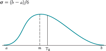
Figure 5-13 The statistical distribution of all possible times for an activity.

In this case, the “6” is not a weighted average but rather an assumption that the range of the distribution covers six standard deviations (6σ). It follows that the variance of this distribution is estimated as

Var = σ² = ((b — a)/6)²

The assumption that the range of the distribution, b — a, covers six standard deviations is important. It assumes that the estimator actually attempted to judge a and b so that 99.7 percent of all cases were greater than a and less than b; that is, less than 1 percent lay outside of these estimates. We have never met a PM who was comfortable with such extreme levels of likelihood. 99.7 percent translates to “almost never outside the range,” (three standard deviations) leading to estimates of a and b that are so small and large, respectively, as to be nearly useless.

But estimators are not so uncomfortable making estimates at the 95 (or 90) percent levels where a is estimated so that 5 (or 10) percent of all cases are less than a, and 5 (or 10) percent are greater than b. These estimates are within the range of everyday experience. These levels, however, do not cover 6σ, so using the above formula for finding the standard deviation will result in a significant underestimation of the uncertainty associated with activity durations and cost estimates. Correcting for such errors is simple. If a and b estimates are made at the 95 percent level, the following should be used to find σ (and squared to find the variance):

σ = (b — a)/3.3

If estimates of a and b are made at the 90 percent level

σ = (b — a)/2.6

The Probabilistic Network, an Example

Table 5-4 shows a set of tasks, their predecessors, and optimistic, most likely, and pessimistic durations for each activity, plus the expected time and activity duration variance. (If the project had been more realistic, that is, much larger, we would have used an Excel^® spreadsheet to handle all the calculations.)

The expected time for each activity was calculated by using the previously noted weighted average of the three time estimates. (The fractional remainders for these calculations are left in sixths for convenience because each T_E will be added to others.) For example, to find T_E for activity a, we have

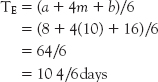
The variance for a is also easily found as

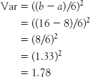
Table 5-4 A Sample Set of Project Activities with Uncertain Durations

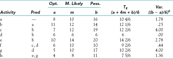
(The traditional ((b — a)/6)² was used to calculate the variance, solely because it is traditional. A problem at the end of this chapter will ask the reader to recalculate the variance assuming 95 and 90 percent estimations, thereby repeating some of the calculations shown in this section.)

The network associated with the data in Table 5-4 appears in Figure 5-14. Note that the entries inside the nodes are the activity identifier, T_E, and variance, in that order. Some activities are known with certainty (i.e., a = m = b), as in task d that takes 6 days in this example. (A real-world example of such an activity would be a 60-day toxicity test of a new drug. In that case, a = m = b = 60 days, not more and not less.) Once in a great while the test may get fouled up and the estimate will be wrong, but our drug manufacturing friends tell us this is quite rare.) In some cases, the optimistic and most likely times are the same, a = m. We might, for instance, allow a specific time for paint to dry, a time that is usually sufficient, but may not be if the weather is very humid. Occasionally, the most likely and the pessimistic times may be the same, m = b, as in f. Sometimes the range may be symmetric, (m — a) = (b — m), but more often it is not. Some activities have little uncertainty in duration, which is to say, low variance. Some have high uncertainty, high variance.

The expected time for each activity can be used to find the critical path and critical time for the network. A forward pass is made, and the critical path is found to be a-b-d-g-h. The critical time is 47 days. Because the mean time (T_E) is used for all activities, there is a 50–50 probability of completing the project in 47 days or less—and also, 47 days or more. Activity slack is calculated by using a backward pass, exactly as we did in the previous section.

There are several problems with conducting the risk analysis in the way that we are demonstrating. For example, given the uncertainty in path durations, we cannot be sure that a-b-d-g-h is actually the critical path. One of the other paths, a-b-c-f, for example, may turn out to be longer when the project is actually carried out. Remember that a, m, and b are estimates, and remember also that the durations are ranges, not point estimates. We refer to a-b-d-g-h as the critical path solely because it is customary to call the path with the longest expected time the “critical path.” Again, only after the fact do we know which path was actually the critical path. The managerial implication of this caveat is that the PM must carefully manage all paths that have a reasonable chance of being the actual critical path. It is also well to remember that in reality all projects are characterized by uncertainty. Sometimes, with routine maintenance projects, for example, activity variances are quite small, but they are rarely zero.

There are also problems with conducting the same type analysis by use of simulation. We will delay discussions of the assumptions behind these methods and a comparison of the pros and cons of such analyses until we have completed descriptions of both methods. In the meantime, it is helpful to bear in mind that the analysis started in Table 5-4, and continued in Table 5-5, and the simulation methods we then discuss are simply two different methods of accomplishing essentially the same thing.

Table 5-5 An MSP Version of a Sample Problem from Table 5-4

Once More the Easy Way

Just as it did for the deterministic sample network, MSP can easily handle the probabilistic network, though as we will see, it does not do some of the calculations that we demonstrate. Those can be done easily enough in Excel^®. The stochastic (a fancy synonym for “probabilistic,” from the Greek word for “conjectural” and pronounced “sta kas' tic” or “stō kas' tic”) network used for the preceding discussion is shown as a product of MSP. Table 5-4 becomes MSP Table 5-5, and Figure 5-14 becomes MSP Figure 5-15.

While Figure 5-14 shows the total elapsed time from Day 0 to Day 47 as one proceeds from left to right, the MSP equivalent, Figure 5-15, shows time as start and finish calendar dates. The project starts on February 4 and is completed on April 10. That is a total elapsed calendar time of 67 days. The time appears significantly different from the 47 days that we determined above as being the expected time for the project. The difference is caused by the fact that MSP assumes (defaults to) a 5-day work week. If you count out the work days on a calendar, you may find that the project seems to take 48 or even 49 days, not 47. That anomaly results from the fact that MSP operates on a real-world calendar. It remembers that February has a national holiday, President's Day. It also remembers that February has 29 days on leap years, and it was on a leap year that we created this example. (It is not difficult to change the work week assumption or to add or delete holidays.) Not counting Saturdays, Sundays, holidays, and remembering the leap year, the project has an expected duration of 47 days, as we thought it should.

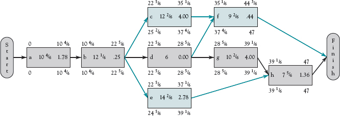
Figure 5-14 An AON network from Table 5-4.

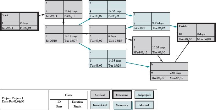
Figure 5-15 An MSP version of a sample problem network in Figure 5-14.

Table 5-6 shows a project plan for development and approval of a project proposal directed to the YMCA for sponsoring a day care service. The project plan covers the process from the investigation of the need for the service through the creation of an implementation plan, given that the YMCA accepts the proposal. In addition to the a, m, and b results, the personnel resource requirements for each activity are shown.

The network for this project appears in Figure 5-16. Note that there is no Start or Finish node, but they are not needed because the start and finish dates for each activity are shown in the activity nodes. In addition to the network, the project calendar for the period from April 16 to May 27 is also shown; see Figure 5-17. This view simply shows the relevant project activities laid out on a standard calendar.

The Probability of Completing the Project on Time

Let us now return to our sample problem of Table 5-4 and Figure 5-14. Recall that the project has an expected critical time of 47 days (i.e., path a-b-d-g-h). How would you respond if your boss said, “The client just called and wants to know if we can deliver the project on April 30, 51 working days from today. I've checked, and we can start tomorrow morning.”

Table 5-6 Three-Time Duration Example for a Day Care Project, with T_E and Resources Shown (MSP)

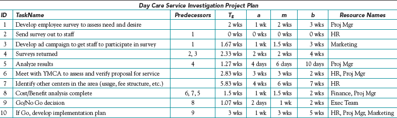
Figure 5-16 A PERT/CPM network for the day care project (MSP).

You know that path a-b-d-g-h has an expected duration of 47 days, but if you promise delivery in 47 days there is a 50 percent chance that this path will be late, not to mention the possibility that one of the other three paths will take longer than 47 days to complete. That seems to you to be too risky. Tomorrow morning will be 50 working days before April 30, so you wonder: What is the probability that the project will be completed in 50 days or less?

This question can be answered with the information available concerning the level of uncertainty for the various project activities. First, there is an assumption that should be noted. The individual variances of the activities in a series of activities (such as a path through a network) may be summed to find the variance of the set of activities on the path itself, if the various activities in the set are statistically independent. In effect, statistical independence means the following in this example: If a is a predecessor of b, and if a is early or late, it will not affect the duration of b. Note what this does not say. It does not say that the date when b is completed will not be affected. If a is late, b is also likely to be late, but the time required to accomplish b, its duration, will not be affected. This may be a subtle distinction, but it is important because the condition of statistical independence is usually met by project activities, and this allows us to answer the boss's question seriously.

There are times when the assumption of statistical independence is not met. For example, assume two activities require some software code to be written. If during the project the code writer originally assigned to the project becomes unavailable and a less experienced code writer is assigned to the tasks, the times to complete these two tasks are clearly not independent of one another. If the lack of experience increases the task time and/or variance of one task, it is likely to impact other tasks in the same fashion. In this case, one should deal with the problem by reestimating the duration of both tasks. In general, this should be done anytime the resources supplied to a project are different from those presumed when the duration of project activities was originally estimated.

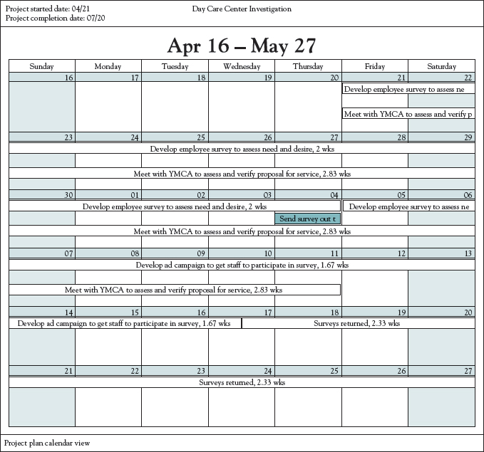
Figure 5-17 An MSP project calendar for the day care project, for the period 4/16 to 5/27.

To complete a project by a specified time requires that all the paths in the project's network be completed by the specified time. Therefore, determining the probability that a project is completed by a specified time requires calculating the probability that all paths are finished by the specified time. Then based on our assumption that the paths are independent of one another, we can calculate the probability that the entire project is completed within the specified time by multiplying these probabilities together. Again, recall from basic statistics that the probability of multiple independent events all occurring is equal to the product of each event's individual probability of occurrence.

To begin, let's evaluate the probability that path a-b-d-g-h, which is apparently the critical path, will be completed on or before 50 days after the project is started. We can find the probability by finding Z in the following equation:

where:

The exact nature of Z will become clear shortly. Using the problem at hand, μ = 47 days, D = 50 days, and = 1.78 + .25 + .00 + 4.00 + 1.36 = 7.39 days. (The square root of 7.39 = 2.719.) Using these numbers, we find

Because the square root of the variance of a statistical distribution equals the standard deviation of that distribution, Z is the number of standard deviations separating D and μ. The distribution in question is the distribution of the times required to complete the path a-b-d-g-h. Consider all possible combinations of the activity times of the tasks on this path. This would include all possibilities from a combination of all optimistic times to a combination of all pessimistic times and everything in between. And even this does not include the highest and lowest project duration outcomes because the estimates do not cover 100 percent of all possible activity times; they cover only 99 + percent. We can illustrate the frequency distribution of the critical path completion times in Figure 5-18. (The Central Limit theorem allows the use of a normal distribution.)

The calculation of Z made above shows the desired date, D, to be approximately 1.1 standard deviations above the expected critical time, μ, for the project. If we define the total area under the curve as 1.0 (100 percent of all times), then the area under the curve to the left of 50 days is equivalent to the probability that the path a-b-d-g-h will be completed in 50 days or less.

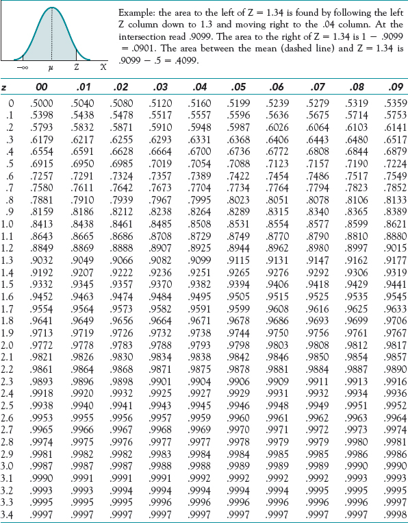
Table 5-7 shows the probability associated with a wide range of values of Z. For Z = 1.10, the probability is .8643 or about 86 percent that this path will be finished on or before Day 50. Again, we remind you that because of uncertainty, other paths may turn out to be critical, possibly delaying the project. Therefore, calculating the probability that the entire project is completed by some specified date requires calculating the probability that all paths that comprise the project are finished by the specified time.

Similar calculations are next done for paths a-b-c-f, a-b-e-h, and a-b-d-f. The probabilities of each of these paths being completed by Day 50 are 98.5 percent, 97.8 percent, and virtually 100 percent, respectively. Based on this, the probability that the entire project is completed by Day 50 is calculated as .864 × .985 × .978 × 1.000 = .832 or 83.2 percent.

A few comments are relevant at this point. First, to simplify the task of calculating the probability that a project is completed by a specified time, for practical purposes it is reasonable to consider only those paths whose expected completion times have a reasonable chance of being greater than the specified time. For example, if the sum of a path's expected time and 2.33 of its standard deviations is less than the specified time, then the probability of this path taking longer than the specified time is quite small, less than 1 percent (2.06 standard deviations would be less than 2 percent). We simply assume that there is a negligible probability that the path will cause the project to be late. For example, path a-b-d-f's expected time and standard deviation are 38.2 and 1.57, respectively. Using this rule of thumb, we get 38.2 + (2.33 × 1.57) = 41.9, which is much less than 50. Since there is less than a 1 percent chance this path will take longer than 41.9 days, there is no need to consider the possibility that it will take longer than 50 days.

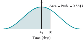
Figure 5-18 The statistical distribution of completion times of the path a-b-d-g-h in Table 5-4.

Table 5-7 The Cumulative (Single Tail) Probabilities of the Normal Probability Distribution (Areas under the Normal Curve from – ∞ to Z)

Second, to calculate the probability that a project will take longer than any specified time, we must first calculate the probability that it will take less than the specified time. Subtracting that probability from 1 gives us the probability that it will take longer than the specified time.

Finally, Excel^®'s NORMDIST function can be used as an alternative to Table 5-7 for calculating the probability that a path finishes by a specified time, D. The syntax of this function is as follows:

To illustrate, the probability that path a-b-d-g-h is completed on or before 50 days can be calculated with Excel^® as = NORMDIST (50, 47, 2.719, TRUE).

Selecting Risk and Finding D

We can also work this problem backwards. Assume that a client is very important, very demanding, and will be very upset if the project is late. The client has asked when the project output will be available. The client insists on a firm date. How sure do you wish to be about being on time? (Don't say 100 percent because that implies a time so long that no one will believe you.) Carefully considering the matter, you decide that you want a 95 percent probability of meeting your promised completion date. When should you tell the client to expect delivery?

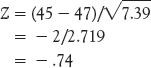
This is the same problem solved just above, but now D, the desired date, is the unknown while the probability associated with Z is preset at .95. Referring to Table 5-7 we can see that for a .95 probability, Z will have a value of 1.645. Therefore,

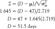
Say, noon of the 52nd day. Note, this result indicates that there is a 95 percent chance of completing path a-b-d-g-h in 51.5 days. Remember that this does not mean that there is a 95 percent chance of completing the entire project in 51.5 days.

We can arrive at the same answer using the Excel^® NORMINV function. The syntax of this function is

= NORMINV (probability, μ, σ_μ)

In our example, this function would be used as follows:

= NORMINV (.95, 47, 2.719)

The Case of the Unreasonable Boss

What happens if your boss is unreasonable, a “pointy-hair” type who insists that he wants the project we have been discussing delivered in 45 days instead of the later delivery times we have considered thus far? To find the likelihood that you can deliver, we return to Z.

In this case,

Reference to Table 5-7 reveals that there are no negative Zs. This merely indicates that D is less than μ. A glance at Figure 5-18 will show this because −.74 is to the left of μ. To find the probability associated with a negative Z, we find the probability of Z as if it were a positive number—for Z = .74. Because Table 5-4 is based on a normal distribution which is symmetric, the negative Z will be as far below m as the positive Z is above it. Therefore, for a negative number the probability will be 1 minus the probability for the same positive number, P(− Z) = 1 — P(Z). The probability for Z = .74 is .77 and thus the probability of Z = −.74 is (1 — .77) = .23. (With Excel^®'s NORMDIST and NORMINV functions, this transformation is not required.) As the PM—other things being the same—you have between a 1 in 4 and a 1 in 5 chance of completing the project on time, not very good odds. The weasel words “other things being the same” will be removed in the next chapter when we reconsider the problem of the pointy-haired boss.

The Problem with Mergers

We are not, of course, writing of big businesses joining to get bigger, but of paths in a network that merge. When two or more paths through a network join, even at the end of the network, paths that have little slack or high variance may become critical simply by chance. For example, examine path a-b-c-f in Figure 5-14, a path with an expected duration of 44.5 days and a path variance of 6.47 days. What is the chance that this path will be longer than our expected project completion time of 47 days?

As we noted earlier, elementary probability theory (see Appendix A) states that if the probability of event A occurring is P(A) and the probability of event B occurring is P(B), then the probability of both events A and B occurring is P(A) × P(B), assuming the events are independent. Tasks a and b are common to both paths, so we ignore them. Tasks d, g, and h have an expected duration of 24.17 days, and their path has a variance of 5.36. Tasks c and f have an expected duration of 21.67 days, and that path has a 4.44 variance. Because d, g, and h have an expected completion time of 24.17 days, there is .5 chance these activities will take longer than 24.17 days. Therefore, we can ask: What is the probability that the c-f path will exceed 24.17 days? Back to Z.

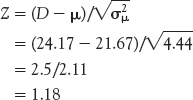
An examination of Table 5-7 shows that for Z equal to 1.18 the probability that the path c-f will be 24.17 days or less is .88. (Using Excel^® we can write = NORMDIST (24.17, 21.67, 2.11, TRUE). The probability that both paths will be 24.17 days or less is .5 × .88 = .44.

It is interesting to remember we began by allowing 50 days for this project and found that the apparent critical path had a .88 probability of being completed in 50 days. What is the likelihood that path a-b-c-f will take longer than 50 days? You can do the arithmetic, but it is approximately equal to .015. So if we have 50 days for the project, we need not worry too much about c-f.

One more problem: Both g and e are predecessors of h. Task g is on the path with the highest expected time, but e is not. What is the chance that e will force h to start late? Because tasks d and e both start at the same time, assuming they both use their ESs, we can ignore their common predecessor, b, in answering this question. If b is not included, we simply compare d-g with e. The path d-g has an expected duration of 16.3 days and a variance of 4.00. Task e has an expected duration of 14.3 days and a variance of 2.78. The question is: What is the probability of e ≥ 16.3 days? Back to Z once again.

Table 5-4 indicates that e will be equal to or less than 16.3 days 88 percent of the time, which means that it will force h to start late only about 12 percent of the time.

The probability that both e and g will be completed by the LS for h (39 1/6 days) is .5 × .88 = .44. The chance that all three paths will be completed in 47 days (T_E for the apparent critical path) is now equal to .50 × .86 × .88 = .38 or slightly less than 40 percent. The chance that all three will be completed by Day 50, the boss's original due date, is still well above 80 percent. The reason for introducing some slack for the entire project is now clear. It should also be clear that given a large project with considerable uncertainty and many paths from start to finish, this manner of dealing with risk is lengthy and probably tedious. More important than tedium, at times the assumption of statistical independence of the paths is not met. There is an alternative way to deal with risk, but it is based firmly on the concepts and issues we have just discussed, so they must be understood before tackling the alternative, simulation.

5.3 SIMULATION

In this section we can take a different approach to managing risk. Specifically, we build on the probabilistic foundation established in the previous section and use simulation to handle the arithmetic as well as help us to understand the consequences of uncertainty. Simulation analysis can provide insight into the range and distribution of project completion times. To illustrate this, once again we use the project activities listed in Table 5-4 and the corresponding network diagram shown in Figure 5-14.

For the purpose of this example, we will make one simplifying assumption. As in Chapter 4, we will assume that the activity times may be reasonably represented by a beta distribution. The spreadsheet shown in Table 5-8 was created to simulate the project.

Table 5-8 Data from Table 5-4 Entered into a CB Spreadsheet with Assumption and Forecast Cells

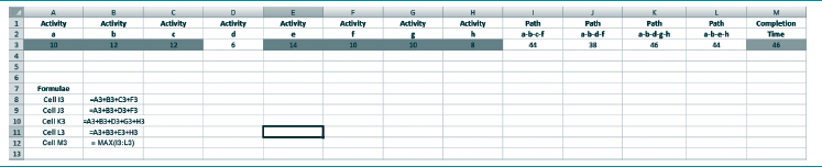
Having opened Excel^® and Crystal Ball^® (CB), we devoted a column to each activity (i.e., columns A through H) and these will be our assumption variables. We then devoted one column (columns I through L) to each path through the network. Finally, we calculate the network Completion Time in column M by taking the maximum value of columns I–L, and this cell becomes our forecast cell. This gives us a very simple model for a complex problem. The hardest part of constructing this model is to identify all paths through the network. On small networks like our example, this is easy. On large networks it may be quite difficult.* Using an MSP PERT network to identify paths can be very helpful.

Reminding the reader that it is easier to follow our instructions if you have the software running, we can now enter data into what becomes Table 5-8.

1. First enter the proper column labels in the first two rows of the spreadsheet, and then enter the most likely time for activity a (from Table 5-4) in cell A3—10 days. CB won't let you define an assumption cell for an empty cell.
2. Click on Define Assumption in the CB ribbon.
3. Click on BetaPERT in the Distribution Gallery and then the OK button.
4. In the BetaPERT Distribution Minimum and Maximum text boxes enter the pessimistic and optimistic times. Note that when you entered the most likely time in step 1, that time already appeared in the BetaPERT Distribution Likeliest text box when it was displayed. Note also that the distribution box assumed pessimistic and optimistic times. Simply click on those boxes and change the times to the ones shown in Table 5-4. When you have done this, click Enter and then OK.
5. Enter the rest of the activity times. Note that activity time for d is a constant. Simply enter “6” in cell D3 and do not use any distribution for the cell.
6. We trust you found the four paths through the network. Identify each path as shown in Figure 5-14 or 5-15, and enter the path duration formulas that simply sum the activity times for each path. (Caution: Recall that the Excel^® copy/paste command will not work, though may appear to do so. Enter the data manually for best results or use the CB copy/paste command.)
7. Now enter the project duration formula in cell M3, that is, = MAX(I3:L3). Click on the cell and then on Define Forecast in the CB ribbon. Label the forecast textbox “Project Completion Time” or whatever you fancy. The Units are “Days.” Click OK. Save the spreadsheet you have created before proceeding with the next step. We will use this spreadsheet again in Chapter 6.
8. If the “Trials” box is not set to 1000, adjust it and then click on the “Start” green arrow. After the run, you will see a statistical distribution similar to Figure 5-19. To view summary statistics, click on the “View” menu option in the Forecast dialog box (see Figure 5-19) and the click on “Statistics” to see a table similar to Table 5-9.

Table 5-9 shows that we made 1000 trials and that the mean project completion time was 47.83 days (in the run made for this writing), the shortest completion time was 41.02 days, and the longest was 55.59 days. Recall that the mean completion time with the analytic approach using the beta distribution was 47 days. The different assumptions about the distribution of the activity times may account for some of the difference between the two estimates of completion time, but most of the difference is probably due to the inclusion of path mergers in the simulation solution. As usual, you can determine the probability that the actual result of the project will have a duration above or below any given time by entering those times in the plus or minus Infinity boxes of the distribution of times; see Figure 5-19.

Figure 5-19 CB frequency chart for project completion time.

Table 5-9 CB summary Statistics for Project Completion Time

Forecast Name	Completion Time
Trials	1,000
Mean	47.83
Median	47.74
Mode	---
Standard Deviation	2.64
Variance	6.99
Skewness	0.143
Kurtosis	2.79
Coeff. of Variability	0.0553
Minimum	41.02
Maximum	55.59
Mean Std. Error	0.08

Incorporating Costs into the Simulation Analysis

In the previous chapter we addressed the topic of budgeting. As you can likely imagine, the cost to complete a project is driven in large part by the time required to complete the project. The longer it takes to complete a task the more resources that are required which in turn leads to greater costs. Furthermore, in a similar fashion to activity durations being uncertain, the cost to complete an activity can be uncertain. For example, the cost to complete an activity may depend on which resources as well as how many resources are assigned to it. Therefore, it stands to reason that we can get a better understanding of the uncertainty surrounding the project's budget by incorporating both schedule and cost uncertainty into our analysis. This is perhaps best illustrated with an example.

For the purpose of our discussion, we extend the analysis conducted in the previous example. More specifically, we supplement the information provided in Table 5-4, with the cost information shown in Table 5-10. As shown in Table 5-10, optimistic, most likely, and pessimistic cost rates have been estimated for each activity. These cost rates are multiplied by the activity duration to determine the cost of the activity. For example, activity A's most likely duration is 10 days (see Table 5-4). At a normal cost rate then, we expect activity A to cost $750 (10 days × $75/day).

Based on the cost estimates provided in Table 5-10, the simulation model shown in Table 5-8 can be enhanced to develop a distribution of potential project costs in addition to the distribution of project completion times as shown in Table 5-11. To develop the enhanced model shown in Table 5-11, the same steps discussed earlier were used to define new Assumption Cells and a new Forecast Cell. More specifically, Assumption Cells for the cost rate of each activity were added in row 7. For the purpose of this example, the cost rates were assumed to follow a triangular distribution. Next, formulas to calculate the cost of each activity were added in row 11. Again, the cost of completing an activity was computed by multiplying its duration in row 3 by its cost rate in row 7. Note that in our enhanced model, we have two sources of uncertainty, namely, the activity durations and cost rates for the activities (except for Activity D, the duration of which is known with certainty). To complete the simulation model, a formula that calculates the cost of the project was added as the sum of activity costs A through H in Cell I11, and then this cell was specified to be a Forecast Cell.

Table 5-10 Sample Set of Project Activities with Uncertain Cost Rates

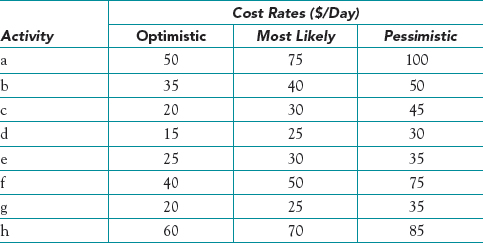
Table 5-11 Simulation Model from Table 5-8 Extended to Analyze Cost of Completing the Project

The distribution of the total cost of the project based on simulating the project 1,000 times is shown in Figure 5-20. Likewise, summary statistics for the total cost of the project are shown in Table 5-12. As can be observed from Table 5-12, the analysis suggests that the project is expected to cost $3,606.76 with a range of $2,646.95 to $4,338.51.

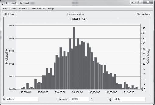
Figure 5-20 CB Frequency Chart for Project Total Cost.

Table 5-12 CB Summary Statistics for the Total Cost of the Project

Traditional Statistics vs. Simulation

At many conferences and in the literature of project management, there are sessions devoted to risk management. The participants at one recent conference, all highly experienced PMs from several different industrial sectors, were not of a single mind about the optimum way to handle the problems we have discussed in this chapter. Some favored the traditional statistical approach, some favored simulation, and some favored adding sizable contingency allowances in both the budget and the schedule, and then ignoring uncertainty. A decade ago, the group that ignored uncertainty would have been in the majority, but they were the smallest of the three groups at this discussion. Dealing with risk is no longer the esoteric interest of a few statisticians, but is now an everyday problem for the PM.

The major difficulty is making sure that the risk analyst understands risk analysis. Irrespective of how the arithmetic is performed, by human or machine, the analyst must understand the nature of the calculations, what they mean and what they do not mean. Conducting a risk analysis by examining the many paths through a large network, and finding those that may turn out to be critical or near-critical, can be an overwhelming task. There may be hundreds or thousands of activities and dozens of paths to be examined. Simply identifying the paths is a daunting job.

Some Common Issues There are a number of issues associated with either the statistical approach or simulation. With an important exception we note just below, both procedures assume that task durations are statistically independent. As we noted above, this might not be the case when resources are shared across the tasks, but the problem can be handled by re-estimating task durations based on the altered resource. Second, with the same exception, both procedures assume that the paths are independent.* Even when paths have tasks in common, the common task durations (and variances) are the same for every path in which they are an element during any given estimate of path duration by whatever procedure. It is as if a constant is being added to each path.

The exception we mention is that simulation has a direct way of circumventing the assumption of statistical independence if the assumption is not realistic. With simulation, one simply includes the activity or path dependencies as a part of the model. The dependencies are modeled by expressing the functional relationship between the activities or paths along with its distribution, mean, and variance so that it may become a variable in the simulation. While this can be done in the statistical approach also, it is much more difficult to handle.

Using the statistical process, the analyst must find the T_E and variance for each path. Using simulation, the computer selects a sample from the distribution of activity times for each activity and then calculates the path duration for each path enumerated.

On the other hand, no matter which method is used, it is rarely necessary to evaluate every path carefully. In a large network, many paths will have both short duration and low variance when compared to high duration paths. Even when it is technically possible for one of the short paths to be critical, it is often very unlikely. For example, consider the path a-b-d-f in our example. It shares activities a, b, and d with a-b-d-g-h, the path with the longest T_E. Activity f has a pessimistic time of 10 days. Activities g and h have optimistic times of 5 + 4 = 9 days. What is the probability that f will take on its maximum value at the same time that both g and h take on their minimum values so that a-b-d-f will be longer than a-b-d-g-h, not to mention simultaneously longer than the remaining two paths? Given that these estimates were made at the ±3σ limit, the probability of g or h being at or below their optimistic estimates is (1 − .9987) = .0013 for each. It is the same for f being at or above its pessimistic estimate. These three things must happen at the same time for a-b-d-f to be longer than a-b-d-g-h. The probability is .0013³ = .000000002. That probability is not zero, but most PMs will not spend time and effort worrying about it. Even when estimates of the optimistic and pessimistic times, a and b, are made at the 90 percent level, the chance that the activities on these particular paths will simultaneously take on their high or low extreme values is about one in a thousand.

The PM will discover the duration of each activity when, and only when, the activity is completed, which is to say after the fact, regardless of the method used to estimate and calculate project duration. Dealing with activity duration as certain does not make it so. We cannot know which of the paths will take the longest time to complete until the project is actually completed. And because we cannot determine before the start of the project which path will be critical, we cannot determine how much slack the other paths will have. We can, however, often make reasonable estimates. We can put our managerial efforts on the activities and paths most likely to require our efforts.

Simulation Because of the computational effort required by the statistical method, we recommend simulation as the preferred tool for risk analysis—after, and only after, the analyst understands the underlying theory of the analysis.

We have included Crystal Ball^® with this book because it is user-friendly software that can be used to facilitate and enhance the simulation of the project networks as well as simulate a wide variety of other types of problems. In addition to the uses we have demonstrated, CB can also facilitate the task of selecting the best distributions to be used to model alternative activities if historical data are available for these activities. Likewise, CB can determine the best distribution to use to characterize project completion times and other outputs of the simulation analysis. Furthermore, it has a comprehensive set of probability distributions available and the selection of these distributions is facilitated by graphically showing the analyst the shape of the distribution based on the parameters specified. This capability allows the user to interact with the software when specifying the parameters of a distribution. The analyst can immediately assess the impact that alternative parameter settings have on the shape of the distribution. Another powerful feature of Crystal Ball^® is its ability to quickly calculate the probability associated with various outcomes such as the probability that the project can be completed by a specified time. In addition, CB can display the results in a variety of formats including frequency charts, cumulative frequency charts, and reverse cumulative frequency charts. It also provides all relevant descriptive statistics as was illustrated earlier.

5.4 THE GANTT CHART

Henry Gantt, a major figure in the “scientific management” movement of the early twentieth century, developed the Gantt chart around 1917. A Gantt chart displays project activities as bars measured against a horizontal time scale. It is the most popular way of exhibiting sets of related activities in the form of schedules.

The Chart

Figure 5-21 shows a Gantt chart of the sample project in Table 5-4. The expected times are used in this illustration. Clearly, Gantt charts are easy to draw. Because task names are usually descriptive, each task shows its name, WBS number, or ID number in order to identify predecessors. Any activity that has no predecessors starts at the beginning of Day 1 and extends to its duration (as in task a). An activity with predecessors begins when its latest predecessor has been completed (as in task f or h).

Problems in understanding the chart can arise, however, when several tasks begin at the same time and have the same duration. If one such task is on the critical path and the others are not, it may be difficult to find the critical path on a Gantt chart. For instance, had c and d both been the same duration, it would not have been possible to tell which was predecessor to f and which to g, just by looking at the chart. This is only a problem when the Gantt chart is prepared manually. Most software, MSP included, will use arrows, bolded bar outlines, colored boxes, or some other visible means of marking the critical path on a Gantt chart as in Figure 5-22.

Even with software aid, the technical dependencies are harder to see on a Gantt chart than on a PERT/CPM network. On the network, technical dependencies are the focus of the model. As can be seen in Figure 5-22, information can easily be added to the chart to show such things as ES, EF, LS, LF, and slack.

Figure 5-21 A Gantt chart of a sample project in Table 5-4 (MSP).

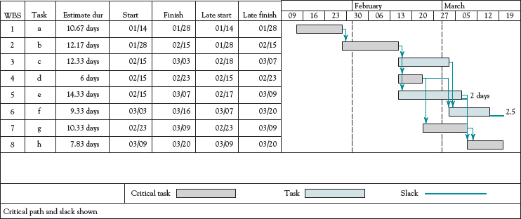
Figure 5-22 A Gantt chart of the sample project in Table 5-4 showing critical path, path connections, slack, ES, LS, EF, and LF (MSP).

Selecting another example for illustration purposes, it is simple to show resource requirements as in the Day Care project (see Table 5-6). The three-time estimates can be shown in Figure 5-23 as well as in Table 5-6, but Figure 5-23 shows only T_E to save space. Time and resource requirements may also be automatically transferred to the Gantt chart if desired.

It is also easy to show the current status of a project that is partially complete, as in Figure 5-24. This project was started on April 21, and its progress is being measured as of June 6. (The calendar dates shown as column titles above the bars indicate the first day of the period, in this case, 4 one-week periods.) Note that Activity 4 starts 1½ days late. It was scheduled to start at midday on May 17, but did not begin until May 19. Activity 4 finishes a week late. If nothing is done to correct the matter, and if nothing happens to increase the lateness, the project will finish about a week late.

Figure 5-23 A Gantt chart of a day care project showing expected durations, critical path, milestone, and resource requirements (MSP).

Figure 5-24 A progress report on a day care project showing actual progress vs. baseline (MSP).

Software such as MSP makes it easy to use a Gantt chart or network to view critical tasks and paths of a project. One can even experiment with adjustments to the project—play “what if' with the project schedule, immediately observing results of the experiments on the screen. At times the PM may question an estimate of task duration, or of the a, m, and b time estimates, submitted by a member of the project team. It is simple to enter alternate time estimates and instantly see the impact on project duration. Of course, this can also easily be done using MSP's PERT network and using simulation.

A great deal of information can be added to Gantt charts without making them difficult to read. A construction firm of our acquaintance added the following symbol to activities that were slowed or stopped because of stormy weather . They used other symbols to indicate late deliveries from vendors, the failure of local government to issue building permits promptly, and other reasons why tasks might be delayed. Milestone symbols—diamonds, , in MSP—are added to the charts, with different shading or color to differentiate between “scheduled” and “completed” milestones. MSP is limited only by the PM's imagination in what can be shown on a network, Gantt chart, or in a project plan.

The major advantage of the Gantt chart is that it is easy to read. Such charts commonly decorate the walls of the project office (or “war room”). They can be updated easily. This is both the strength and the weakness of the Gantt chart. Anyone interested in the project can read a Gantt chart with little or no training—and with little or no technical knowledge of the project. This is the chart's strength. Its weakness is that to interpret beyond a simplistic level what appears on the chart or to alter the project's course may require an intimate knowledge of the project's technology—not necessarily visible on the chart, but available on the network or the project plan. Not uncommonly, the Gantt chart is deceptive in its apparent simplicity.

We should add that one must be cautious about publicly displaying Gantt charts that include activity slack, or LSs and LFs. Some members of the project team may be tempted to procrastinate and tackle the work based on the LS or LF. If done, this makes a critical path out of a noncritical path and becomes an immediate source of headaches for the PM who, among other things, loses the ability to reschedule the resources used by tasks that once had slack. Senior managers have even been known to view activity slack as an invitation to shorten an entire project's due date. We recommend caution and careful education of the boss.

At base, the Gantt chart is an excellent device to aid in monitoring a project and/or in communicating information on its current state to others. Gantt charts, however, are not adequate replacements for networks. They are complementary scheduling and control devices.

5.5 EXTENSIONS TO PERT/CPM

There have been several extensions to both network and chart forms of project scheduling. At times these extensions are quite sophisticated; for example, the application of fuzzy set theory to aid in estimating activity durations in cases where activity durations are difficult to estimate because project activities cannot be well defined (McMahon, 1993). In this section we briefly discuss one significant extension of traditional scheduling methods, precedence diagramming. (Elihu Goldratt's Critical Chain (1997) is also a significant addition to traditional scheduling methods. It uses networks that combine project scheduling with resource allocation. It is discussed in Chapter 6 on resource allocation.)

Precedence Diagramming

One shortcoming of the PERT/CPM network method is that it does not allow for leads and lags between two activities without greatly increasing the number of subactivities to account for this. That is, our regular network methods described earlier assume that an activity can start as soon as its predecessor activities are completed. Sometimes, however, the restrictions are more complex—for example, when a follow-on activity cannot begin until a certain amount of time after (or even before) its predecessor is completed (or sometimes started). For instance, a successor may have to wait for paint to dry or cement to harden. In this case, we might add a fictitious activity after painting or pouring the cement that takes the required time (but no resources) and then let the follow-on begin. For a leading activity, we might break the predecessor activity into two activities a followed by b and let the follow-on start after a is completed and operate in parallel with b, the remainder of the predecessor activity. In construction projects, in particular, it is quite common for the following restrictions to occur. (Node designations are shown in Figure 5-25.)

• Finish to Start Activity 2 must not start before Activity 1 has been completed. This is the typical arrangement of an activity and its predecessor. Other finish-start arrangements are also possible. If the predecessor information had been written “1 FS + 2 days,” Activity 2 would be scheduled to start at least 2 days after the completion of Activity 1, as shown in Figure 5-25. For instance, if Activity 1 was the pouring of a concrete sidewalk, Activity 2 might be any activity that used the sidewalk.

  

  Figure 5-25 Precedence diagramming conventions.

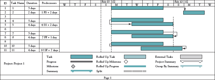
• Start to Start Activity 5 cannot begin until Activity 4 has been underway for at least 2 days. Setting electrical wires in place cannot begin until 2 days after framing has begun.
• Finish to Finish Activity 7 must be complete at least 1 day before Activity 8 is completed. If Activity 7 is priming the walls of a house, Activity 8 might be the activities involved in selecting, purchasing, and finally delivering the wallpaper. It is important not to hang the paper until the wall primer has dried for 24 hours.
• Start to Finish Activity 11 cannot be completed before 7 days after the start of Activity 10. If Activities 10 and 11 are the two major cruising activities in a prepaid weeklong ocean cruise, the total time cannot be less than the promised week. The S–F relationship is rare because there are usually simpler ways to map the required relationship.

Precedence diagramming is an AON network method that easily allows for these leads and lags within the network. MSP handles leads and lags without problems. Network node times are calculated in a manner similar to PERT/CPM times. Because of the lead and lag restrictions, it is often helpful to lay out a Gantt chart to see what is actually happening. Most current project management software will allow leads, lags, delays, and other constraints in the context of their standard AON network and Gantt chart programs.

Final Thoughts on the Use of These Tools

Three decades ago it was common to hear, “No one uses PERT or CPM.” It was not true. One decade ago we heard, “No one uses that probability stuff.” It was not true. We even heard, “No one uses ______ computer package,” which was also untrue. These statements were not true a decade ago—and they are even less true (if that is semantically possible) today. Current software makes it easy to use networks and Gantt charts. Current software handles three-time estimates of duration and can do all the calculations almost instantly. Current software makes simulation a straightforward procedure.

Excel^® and other popular spreadsheets can calculate variances and find expected times. MSP can do some of these calculations, but not others. MSP does not find the standard deviation or variance of three-time duration estimates and cannot find the probability of completing a task or the entire project within a given time limit. Probability calculations are, however, easily handled by simulation. The analyst, of course, must examine the paths, and select those for further analysis. The software can do the arithmetic, but the analyst must enter the appropriate numbers and ask for the appropriate calculations for each path to be analyzed, and then find the probabilities. With large networks, this will probably be a massive and tedious task. On the other hand, it is almost never required to enumerate and evaluate all paths in a simulation—even if simulation could do so rapidly.

As we have noted several times, the same arguments and methods are appropriate for managing uncertainty in resource usage and preparing project budgets. The calculations and simulations are the same as those used with task and project duration.

When struggling with risk analysis and management, it is well to remember why the PM must engage the struggle. The PM is responsible for keeping the project within its budget and on time. This chapter is devoted to developing the information the PM requires to meet these responsibilities. The PM does not manage the project as a totality; rather he or she manages the specific tasks and subtasks that make up the project. The methods introduced above are intended to help the PM understand precisely where management effort is needed.

As we noted briefly above, it is relevant to point out that identifying one or more paths as critical might actually be detrimental to project performance—if the PM is not managing the project team as well as the project. If the PM is not alert to the possibility, activity slack may lead to neglect of noncritical activities. As Parkinson teaches us, work tends to fill the time allowed, and activities lose their slacks. For example, non-critical paths may slip far enough behind schedule that they become critical—simply because the project team perceives them to be of low priority. At the same time, the apparently critical path may finish ahead of schedule because of the extra management attention it receives.

Goldratt (1997, Ch.13) refers to other causes of project delay resulting from “human nature.” There is, for instance, the “student syndrome.” Given the deadline for a homework assignment, students often plead for more time. Given more time, many simply postpone starting the assignment. Goldratt also reminds us that if a task is finished early, its successor tasks are still started when they were originally scheduled. The result is that delays resulting from tasks finishing late are not offset by the potential gains from those that finish early. There is also the fact that “five plus five equals thirteen.” If one team member estimates that one task will require 5 days and a second team member estimates that a successor task will require 5 days, the boss then estimates that the pair will require 13 days—just to be safe. The work, of course, will expand to require at least 13 days.

If the PM becomes entranced with the technology of the project and fails to manage the project team, the team itself can become confused and frustrated as the reality of the project unfolds. Today's path-slack disappears and a new critical path is born—only to change tomorrow when some other path becomes critical. In such cases, and they are common in reality, it is not easy to remind oneself that recognizing and analyzing uncertainty does not cause uncertainty—nor does it cause uncertainty to disappear. The PM's job includes teaching project team members enough about risk that they can understand its nature and, thereby, cooperate in developing ways to deal with it.

At this point, it is helpful to remember that there are problems for which risk analysis, by whatever method, is probably not required. Routine maintenance and routine construction projects are among such cases—unless the projects are quite large or have not been performed recently. In most such projects the routine character of the work means that the variances of task durations are quite small and the cost of carrying out a careful risk analysis is rarely justified.

In the next chapter, we turn our attention to resource allocation and the problems of controlling the use and flow of resources. We also deal with the issue of integrating schedule and budget by examining the nature of time-resource trade-offs.

    REVIEW QUESTIONS

1. How would a PM manage critical path tasks differently than noncritical path tasks?
2. How is slack determined?
3. How do you determine the ES for an activity with two predecessors? How do you determine the LF for an activity with two successors?
4. Will all the activities on a noncritical path have the same slack? Why or why not?
5. For the following project,

   (a). List all predecessors of task 5.

   (b). List all predecessors of task 4.

   (c). List all predecessors of the network finish (F).

   

6. What is a “dummy” activity?
7. Consider Figure 5-14. Paths a-b-c and a-b-d converge at activity f, but we ignored this potential merge problem in the text. Why?
8. What is meant by “project slack”?
9. When using AON networks, how does one indicate an event such as a project milestone?
10. A probabilistic network has a critical path of 21 days and a .95 probability of completing this path in 24 days. Therefore, the project has a .95 chance of being finished by the end of the 24th day. True or False? Briefly explain your answer.
11. “Not uncommonly, the Gantt chart is deceptive in its apparent simplicity.” Briefly explain.
12. When activity times are known with certainty, the critical path is defined as the set of activities on a path from the project's start event to its finish event that, if delayed, will delay the completion date of the project. Why must this definition be modified in situations where the activity times are not known with certainty? Are there any dangers associated with not modifying the definition?

    DISCUSSION QUESTIONS

13. How might you use the network approach to help prepare cost estimates?

14. When would it be accurate to determine the probability of project completion by multiplying the probabilities of all the paths through the network together? When would it not be accurate?

15. Reconsider Question 14. If this approach is not accurate, would the probability of completion considering the critical path alone be more accurate? How might you estimate the correct probability without resorting to simulation?

16. Why do you think most PMs use MSP's Gantt chart format (see Figure 5-22) more commonly than the network format?

17. Which of the linkages in precedence diagramming do you think is most commonly used? Why?

18. In the calculation of variance for optimistic and pessimistic activity duration estimates made at the 95 or 90 percent level, the denominator of the fraction that approximates the standard deviation of the time distribution changes from the traditional (b — a)/6 to (b — a)/3.3 for 95 percent and to (b — a)/2.6 for 90 percent. Where did the 3.3 and the 2.6 come from?

19. Given all the estimating done to determine the duration of project activities, what does it mean to say that “only after the fact do we know which path was actually the critical path?”

20. It was noted that “the PM must manage the project team as well as the project.” Explain why.

21. Why do you think scheduling has been the major focus of effort throughout the history of project management rather than performance or budgeting?

    PROBLEMS

22. Refer to the network in Figure 5-14. What is the probability that path a-b-c-f will interfere with the promised project completion of 50 days? Recall that the critical path, a-b-d-g-h, had a probability of .86 for a 50-day completion. What is the probability that both paths will be complete in 50 days?

23. Refer to Table 5-4 and Figure 5-14. Recalculate the variance for each activity on the assumption that the optimistic and pessimistic estimates were made with a 95 percent probability. Recalculate the probability that the critical path will be completed in 50 days.

24. Refer to Table 5-4 and Figure 5-14. Recalculate the variance for each activity on the assumption that the optimistic and pessimistic estimates were made with a 90 percent probability. Again, recalculate the likelihood that the critical path will be finished in 50 days.

25. Given the information in the following table:

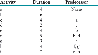
a. Construct the network diagram.

b. Find each activity's ES, EF, LS, and LF.

c. Identify all paths. Which path is the critical path?

d. Calculate the slack for each activity.

e. How long will it take to complete the project?

26. Given the information in the following table, draw the AOA network. Using the same information, enter the data into MSP assuming a 7-day workweek. (To change the calendar in MSP from its 5-day week default, click “Help,” type “calendar change,” and follow directions.) Develop the appropriate AON network and Gantt chart. Using any method you wish, find the critical path and critical time for the network. Then find the slack for all activities.

27. In the following table, task durations are given in weeks. The estimates were made at the 95 percent level (see Section 5.2, Calculating Probabilistic Activity Times subsection).

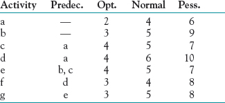
a. Find the expected time and variance for each task.

b. Draw the network (either AOA or AON) and find the critical path and time.

c. Find the probability that the critical path will be completed in 23 weeks.

d. Find the probability that the other main paths will be completed in 23 weeks.

e. What is the probability that the entire network will be completed in 23 weeks?

28. Given an auditing project with the following activities:

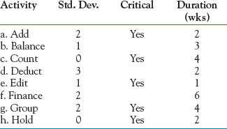
Using the critical path, find:

a. The probability of completing this project in 12 weeks or less, as the client desires.

b. The probability of completing this project in 13 weeks or less.

c. The probability of completing this project in 16 weeks or less, the client's drop-dead date.

d. The number of weeks required to assure a 92.5 percent chance of completion, as guaranteed by the auditing firm.

29. Given the following information regarding a project involving an initial public offering (IPO):

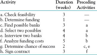
a. Draw the network.

b. What is the critical path?

c. When will the offering be available (end of the project)?

d. What is the effect on the project if activity e (approvals) takes an extra week? Two extra weeks? Three extra weeks?

30. Enter the following information into an Excel^® spreadsheet. The time estimates were made at the 90 percent level (see Section 5.2, Calculating Probabilistic Activity Times subsection). All activity times are in days.

a. Draw the network. (You may use MSP, or draw an AOA or AON network by hand.)

b. Using Excel^®, calculate the expected time (T_E) and variance for each activity.

c. Using the expected times, find the critical path and critical time. (Use the analytic method.)

d. Find the probability that the critical path will be completed in 38 days or less.

e. Are there any serious sources of merge bias? What are they? Calculate the probability of finishing the project on or before day 38 when merge bias is included.

f. Assume that the times in the table were made on the 99+ percent level. Recalculate the activity variances with this assumption and find the probability that the critical path will be complete in 38 days. (Note, the altered assumption will change activity variance, but not the expected activity durations.) Briefly explain the difference in probabilities.

g. How many days are required for the critical path to have a .9 probability of completion?

31. Given the project in Problem 27, simulate the completion of the project 1000 times, assuming that the activity times follow a normal distribution and that the time estimates are made at the 95 percent level.

a. Determine the probability of each path becoming the critical path.

b. What is the probability that the project is completed in 23 weeks?

c. How do your answers compare with your answers in Problem 27?

32. The project referred to in Problem 31 has been partially completed. Task a required 4 weeks, task b 9 weeks, task c 4 weeks, and task d 5 weeks. Update the simulation model you developed for Problem 31 and calculate the probability that the project will be finished in 23 weeks. Explain why the probability of completing the project in 23 weeks has changed.

33. Given the project in Problem 30, simulate the completion of the project 1000 times, assuming that the activity times are at the 99+ percent level and follow a triangular distribution.

a. Determine the probability of each path becoming the critical path.

b. What is the probability that the project is completed in 32 days? In 34 days? In 38 days?

c. How do your answers compare with your answers in Problem 30?

    DISCUSSION PROBLEM

34. The following activities were listed during a brainstorming session on product development. Find the appropriate predecessor-successor relationships and then construct an AON network to reflect the project using the activity duration times given in the information table. Assume a 5-day workweek. Find the critical path and time for the project. Find the slack for all activities.

1. Organize the sales office: Hire sales manager. (6 weeks)
2. Hire sales personnel: The sales manager will recruit and hire the salespeople needed. (4 weeks)
3. Train sales personnel: Train the salespeople hired to sell the product to the distributors. (7 weeks)
4. Select advertising agency: The sales manager will select the agency best suited to promote the new product. (2 weeks)
5. Plan advertising campaign: The sales office and advertising agency will jointly plan the advertising campaign to introduce the product to the public. (4 weeks)
6. Conduct advertising campaign: The advertising agency will conduct a “watch for” campaign for potential customers. (10 weeks)
7. Design package: Have packaging engineer design the package most likely to “sell.” (2 weeks)
8. Set up packaging facility: Prepare to package the products when they are received from the manufacturer. (10 weeks)
9. Package initial stocks: Package stocks received from the manufacturer. (6 weeks)
10. Order and receive stock from the manufacturer: Order the stock from the manufacturer. The time given includes the time for delivery. (13 weeks)
11. Select distributors: The sales manager will select the distributors whom the salespeople will contact to make sales. (9 weeks)
12. Sell to distributors: Take orders from the distributors for the new product, with delivery promised for the product-introduction date. If orders exceed stock, assign stock on a quota basis. (6 weeks)
13. Ship stock to distributors: Ship the packaged stock to distributors in accord with their orders or quota. (6 weeks)

Question: What managerial problems and opportunities do you see as a result of your work?

    INCIDENTS FOR DISCUSSION

Springville Fire Department

The city of Springville is building a new fire station in their city. The city is expanding and is in need of a second fire station closer to the newer areas of the city to ensure shorter response times. The project manager and the project team have been selected for the project. The team is very interested in selecting the scheduling technique that will be used to follow the project through to completion.

The project manager, city manager, and chief of the fire department have set the following criteria for the process of selecting the scheduling technique: easy to use, shows durations of tasks, shows milestones, can see the flow of work, can see the sequence of events, can depict which tasks can be undertaken at the same time, and can tell how far tasks are from completion. The city manager favors the Gantt chart, the chief likes PERT, and the project manager prefers CPM.

Question: If you were the project manager, which method would you use, and why?

Attack of the Killer Worm

Lee Antoinio was the CIO of a large publishing house. Her network administrator, Andy McPester, came to her one sunny September afternoon and informed her that a worm had attacked their network. It had shut down two of their 45 servers and had potential to harm the other servers as well as the 323 personal workstations throughout the enterprise. Andy knew that he could not report this problem to Lee without a recommended project plan for a solution. Andy and Lee had a good, trusting relationship, but Lee insisted that Andy investigate all options and come to her with the most viable solution to any problem.

Andy's project plan outlined that it would take 30 to 45 minutes to touch each PC to protect them from the worm, and longer if they were already infected. It would take almost an hour to check the other servers and repair them. Andy discussed the time estimates with his desktop staff. Andy proposed paying six staff members overtime to work 4 hours after their normal business day for the next week or two to check each personal workstation. He did not want to affect productivity of the company's staff during the day. Andy proposed repairing the servers the same way with two additional staff members in the evenings. Lee felt that the time estimates and costs were too high. She did not think it would take that amount of time for each machine to get repaired. She was concerned that some of Andy's staff may have overestimated the time needed. She also was not sold on the notion that all the work would be done at night, paying staff overtime.

Question: How would you recommend they reach a consensus on the project plan?

St. Dismas Assisted Living Facility Program Plan—3

The steering team meeting held August 31 went quite well. Fred felt that his team members had worked well together at determining the steps and the associated costs of the program. The CFO presented the program budget first, and then project team members presented their draft project plans.

The COO presented the following project plan:

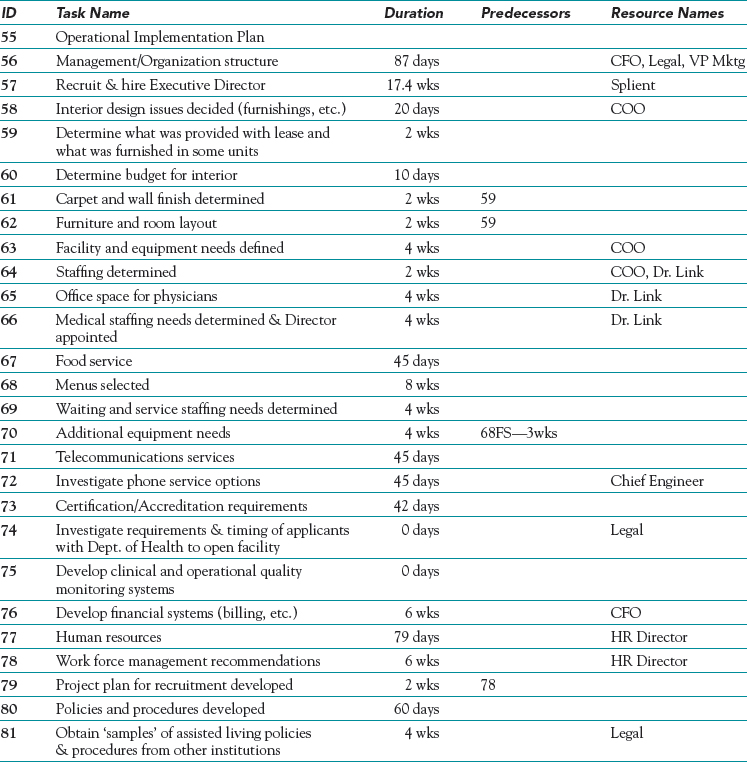
The Chief Legal Counsel for the medical center presented his project plan. Fred had asked him to join the team when it became apparent that there were significant compliance and legal issues associated with this project.

The Vice President of Marketing presented her project plan and stated that she and her staff were responsible for every step in the plan. She was still working with her staff to determine who does what. The Marketing VP made it clear to the team that she needed 5 months for the marketing plan implementation to be able to meet the occupancy requirements at start-up. She restated that her team must have this lead time to the completion of the construction and furnishing phase of the Program.

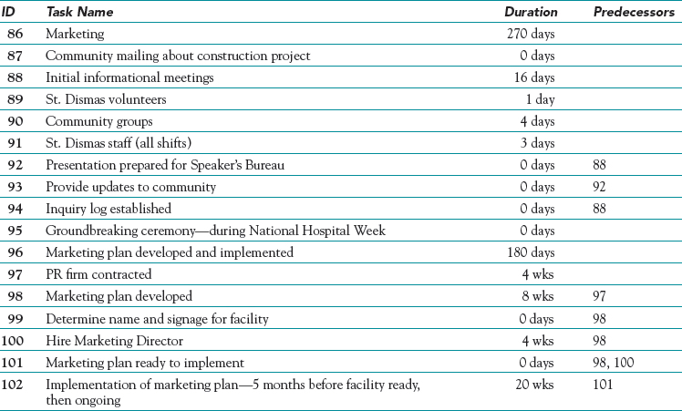
As Fred was explaining that the next job of the group was to complete a final version of all project plans and firm up the schedule of the Program, the Construction Project Manager stated that it was his turn to present his broad project plan for construction of the facility. He also added that he had a major scheduling issue to bring to the team. The Construction Project Manager presented the following broad project plan for facility construction.

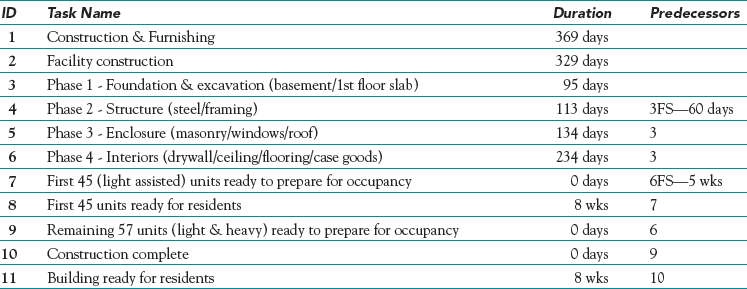
The construction PM proceeded to explain that the scheduling constraints that the Board of Trustees gave the team were not feasible. The Board wanted construction to begin immediately after the elections in November and to be ready for occupants by June. The contractor did not want to begin the project at the beginning of winter. The first phases of the project plan detailed work that needed to be completed outside. If the weather was bad, the construction PM knew the schedule would be affected. The construction project manager also pointed out that the schedule created by the contractor was designed around a 40-hour, 5-day workweek. If the building project began in November, the estimated project duration would be increased by 1 to 2 months, during which time some construction crewmen would have to be paid, thereby increasing the building cost.

The PM recommended that construction begin in February or March of the following year, which would give the facility a shorter build time and a lower cost. The budget and project duration submitted were based on a March 1 start date. He stated that the construction phase of the project did not need to hold up the other members of the Program team— they could begin their work on their projects anytime.

    QUESTIONS

1. Draw a Gantt chart for the construction phase of the program. What is the completion date if construction starts in March? What is the completion date of the project if construction is started in November?
2. Why is it not possible to meet the scheduling constraints set by the Board? What is your recommendation to handle the scheduling problem?
3. When will the program be completed based on your recommendation?
4. Develop a Gantt Chart of the Marketing Plan and Implementation Phase of the Program. Determine the start date of the Marketing Plan project in order to meet your recommended facility ready for occupancy date.
5. What is the next step the team members must take in order to complete their project plans?

NutriStar

NutriStar produces a line of vitamins and nutritional supplements. It recently introduced its Nutri-Sports Energy Bar, which is based on new scientific findings about the proper balance of macronutrients. The energy bar has become extremely popular among elite athletes and other people who follow the diet. One distinguishing feature of the Nutri-Sports Energy Bar is that each bar contains 50 milligrams of eicosapentaenoic acid (EPA), a substance strongly linked to reducing the risk of cancer but found in only a few foods, such as salmon. NutriStar was able to include EPA in its sports bars because it had previously developed and patented a process to refine EPA for its line of fish-oil capsules.

Because of the success of the Nutri-Sports Energy Bar in the United States, NutriStar is considering offering it in Latin America. With its domestic facility currently operating at capacity, the President of NutriStar has decided to investigate the option of adding approximately 10,000 square feet of production space to its facility in Latin America at a cost of $5 million.

The project to expand the Latin American facility involves four major phases: (1) concept development, (2) definition of the plan, (3) design and construction, and (4) start-up and turnover. During the concept development phase, a program manager is chosen to oversee all four phases of the project and the manager is given a budget to develop a plan. The outcome of the concept development phase is a rough plan, feasibility estimates for the project, and a rough schedule. Also, a justification for the project and a budget for the next phase are developed.

In the plan definition phase, the program manager selects a project manager to oversee the activities associated with this phase. Plan definition consists of four major activities that are completed more or less concurrently: (1) defining the project scope, (2) developing a broad schedule of activities, (3) developing detailed cost estimates, and (4) developing a plan for staffing. The outputs of this phase are combined into a detailed plan and proposal for management specifying how much the project will cost, how long it will take, and what the deliverables are.

If the project gets management's approval and management provides the appropriations, the project progresses to the third phase, design and construction. This phase consists of four major activities: (1) detailed engineering, (2) mobilization of the construction employees, (3) procurement of production equipment, and (4) construction of the facility. Typically, the detailed engineering and the mobilization of the construction employees are done concurrently. Once these activities are completed, construction of the facility and procurement of the production equipment are done concurrently. The outcome of this phase is the physical construction of the facility.

The final phase, start-up and turnover, consists of four major activities: pre-start-up inspection of the facility, recruiting and training the workforce, solving start-up problems, and determining optimal operating parameters (called centerlining). Once the pre-start-up inspection is completed, the workforce is recruited and trained at the same time that start-up problems are solved. Centerlining is initiated upon the completion of these activities. The desired outcome of this phase is a facility operating at design requirements.

The following table provides optimistic, most likely, and pessimistic time estimates for the major activities.

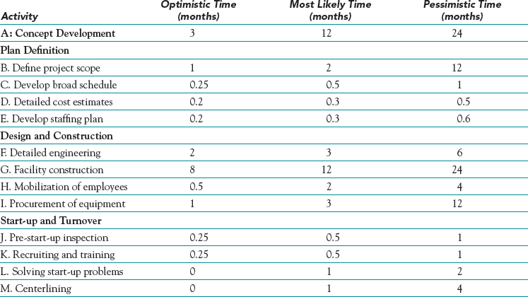
    QUESTIONS

1. Draw a network diagram for this project. Identify all paths through the network diagram.
2. Simulate the completion of this project 1,000 times, assuming that activity times follow a betaPERT distribution. Estimate the mean and standard deviation of the project completion time.
3. Develop a histogram to summarize the results of your simulation.
4. Calculate the probability that the project can be completed within 30 months. What is the probability that the project will take longer than 40 months? What is the probability that the project will take between 30 and 40 months?

Launching E-Collar

Pet Technologies Inc. has completed the development of a revolutionary pet collar code named e-collar. E-collar is designed for dogs and allows pet owners to identify the location of their dog using their smartphones. In addition to purchasing the e-collar, the pet owners must download a free app for their smartphone and pay a small monthly fee that is yet to be determined in order to connect the e-collar to a cellular network.

In the past, Pet Technologies has used the services of Ad Jungle to develop its advertising campaigns. Ad Jungle is located in the same city as Pet Technologies and is a boutique advertising agency with 25 full-time employees and a similar number of people it contracts with on an ad hoc basis. Pet Technologies has reached out to Ad Jungle and has requested an estimate for the cost of developing an advertising campaign for the e-collar.

Ad Jungle begins the process of developing an ad campaign by first meeting with the client to learn about the product to be advertised. Based on what is learned, Ad Jungle works with the client to define the target audience for the advertising campaign. Because the target audience may be different than its current customer base, market research is often required. Historical data suggests that defining the target market typically takes 80 hours (2 weeks). In some cases, determining the target audience is fairly routine and can be done in as little as a day and a half (12 hours in total) while in other cases much less is known about who will use the product and defining the target market can take as long as 4 weeks (160 hours). Also, the number of people working on the task at any one time varies as does their hourly bill rate. Given this, the average amount the customer is billed for the work to determine the target audience typically averages $170 per hour. In some cases, however, the hourly rate was as low as $100 per hour and in other cases as high as $450 per hour.

Once the target audience has been defined, alternative concepts for the advertising campaign are developed. A key aspect of developing the concept is deciding on the tone the campaign will use such as humorous, dramatic, or informative. Concept development is a highly creative process and often requires several iterations between Ad Jungle and its clients. On average, concept development takes 2 weeks (80 hours) but has been completed in as little as 1 week (40 hours) or as long as 5 weeks (200 hours). Only one person from Ad Jungle works on concept development, and typically these employees are billed out at $125 per hour. However, the least experienced employee is billed out at $75 per hour and the most experienced person is billed out at $200 per hour.

Once the client signs off on the concept, the development of the creative collateral (brochures, print ads, scripts for TV commercials, and so on) and determining the mix of media are done concurrently. The amount of time it takes to develop the creative collateral depends on how many media channels will be used (e.g., print, TV, online), how many people are assigned to work on developing the creative collateral, and how much involvement the client wants to have in the process. Typically, developing the creative collateral requires 3 weeks (120 hours) but has been done in as little as 1 week (40 hours) and on other occasions required 6 weeks (240 hours). Furthermore, the number of people and their bill rates varies from project to project. On average, the hourly bill rate for developing the collateral is $275 but has been as low as $145 and as high as $425.

Determining the mix of media is almost always done by the same person at Ad Jungle. This person is currently billed out at $150 per hour. The amount of time it takes to determine the mix of media that will be used ranges from half a day (4 hours) to 2 days (16 hours), but it typically takes 1 day (8 hours).

Once the collateral has been developed and the mix of media determined, the final step is production where the advertising materials are developed. The production of the advertising materials is outsourced to firms, and Ad Jungle assigns one account manager to oversee the work. The account managers are billed out at an hourly rate of $200. On average, 80 hours of the account manager's time is needed to oversee production. In some cases, as little as 30 hours of the account manager's time was required, while in other cases as many as 160 hours were needed.

    QUESTIONS

1. Draw a network diagram for this project. Identify all the paths through the network diagram.
2. Simulate the completion of this project 1,000 times, assuming that activity times and costs follow a triangular distribution. Estimate the mean and standard deviation of the project completion time. Also, estimate the mean and standard deviation of the amount the client would be billed for the project.
3. What is the probability the project can be done for less than $100,000? What is the probability the project will take between 350 and 450 hours?
4. Based on the results of your simulation analysis, how would you respond to Pet Technologies' request for an estimate of the project costs and duration?

    BIBLIOGRAPHY

DE MEYER, A., C. H. LOCH, and M. T. PICH. “Managing Project Uncertainty: From Variation to Chaos.” MIT Sloan Management Review, Winter 2002. (This article provides a useful classification of uncertainty faced in projects and provides specific suggestions for managing each type of uncertainty.)

GOLDRATT, E. M. Critical Chain, Great Barrington, MA, North River, 1997.

HULETT, D. T. “Project Schedule Risk: Monte Carlo Simulation or PERT?” PM Network, February 2000. (Hulett comes to the same general conclusion that we do. Simulation is superior to the statistical methods of PERT for complex problems. In stating his case, however, he fails to note that for a PM to use simulation effectively, the PM should understand the statistics of simulation.)

KAMBUROWSKI, J. “New Validations of PERT Times.” Omega, International Journal of Management Science, Vol. 25, No. 3, 1997.

KEEFER, D. L., and W. A. VERDINI. “Better Estimation of PERT Activity Time Parameter.” Management Science, September 1993.

LAWRENCE, J. A., Jr., and B. A. PASTERNAK. Applied Management Science, New York: Wiley, 1998. (This book has solution techniques for finding the critical path and time for a network using Excel's^® Solver.)

LEACH, L. “Schedule and Cost Buffer Sizing: How to Account for the Bias between Project Performance and Your Model.” Project Management Journal, June 2003. (This article identifies a variety of sources of schedule and cost biases and provides recommendations for coping with them.)

LIBERATORE, M. J. “Project Schedule Uncertainty Analysis Using Fuzzy Logic.” Project Management Journal, December 2002. (Our discussion in this chapter addresses schedule uncertainty from both a probability theory approach and using computer simulation. This article demonstrates the use of fuzzy logic for assessing project schedule uncertainty.)

MCMAHON, C. S. “Using PERT as an Approximation of the Fuzzy-Project Network Analysis.” IEEE Transactions on Engineering Management, May 1993.

MEREDITH, J. R., and S. J. MANTEL, Jr. Project Management: A Managerial Approach, 8th ed., Hoboken, NJ: John Wiley, 2012.

PRITSKER, A. A. B. “Gert Networks.” The Production Engineer, October 1968.

RUSKIN, A. M. “Using Unders to Offset Overs.” PM Network, February 2000.