Probability and Statistics

This appendix is intended to serve as a brief review of the probability and statistics concepts used in this text. Students who require more review than is available in this appendix should consult one of the texts listed in the bibliography.

A.1 PROBABILITY

Uncertainty in project management is a fact of life. The duration of project activities, the costs of various resources, and the timing of a technological change all exemplify the types of uncertainties encountered when managing projects. Each of these random variables is more or less uncertain. Further, we do not know when or if a given activity will be successfully completed, a senior official will approve a project, or a piece of software will run without problems. Each event is more or less uncertain. We do not know the values that each variable and event will assume.

In common terminology we reflect our uncertainty with such phrases as “not very likely,” “not a chance,” “for sure.” While these descriptive terms communicate one's feeling regarding the chances of a particular event's occurrence, they simply are not precise enough to allow analysis of chances and odds.

Simply put, probability is a number on a scale used to measure uncertainty. The range of the probability scale is from 0 to 1, with a 0 probability indicating that an event has no chance of occurring and a probability of 1 indicating that an event is absolutely certain to occur. The more likely an event is to occur, the closer its probability is to 1. This probability definition, which is general, needs to be further augmented to illustrate the various types of probability that decision makers can assess. There are three types of probability that the project manager should be aware of.

• Subjective probability
• Logical probability
• Experimental probability

Subjective Probability

Subjective probability is based on individual information and belief. Different individuals will assess the chances of a particular event in different ways, and the same individual may assess different probabilities for the same event at different points in time. For example, one need only watch the blackjack players in Las Vegas to see that different people assess probabilities in different ways. Also, daily trading in the stock market is the result of different probability assessments by those trading. The sellers sell because it is their belief that the probability of appreciation is low, and the buyers buy because they believe that the probability of appreciation is high. Clearly, these different probability assessments are about the same events.

Logical Probability

Logical probability is based on physical phenomena and on symmetry of events. For example, the probability of drawing a three of hearts from a standard 52-card playing deck is 1/52. Each card has an equal likelihood of being drawn. In flipping a coin, the chance of “heads” is 0.50. That is, since there are only two possible outcomes from one flip of a coin, each event has one-half the total probability, or 0.50. A final example is the roll of a single die. Since all six sides are identical, the chance of any one event occurring (i.e., a 6, a 3) is 1/6.

Experimental Probability

Experimental probability is based on frequency of occurrence of events in trial situations. For example, in estimating the duration for a particular activity, we might record the time required to complete the activity on similar projects. If we collect data on 10 projects and the duration was 20 days on 3 of the 10, the probability of the duration equaling 20 days is said to be 0.30 (i.e., 3/10).

Both logical and experimental probability are referred to as objective probability in contrast to the individually assessed subjective probability. Each of these is based on, and directly computed from, facts.

A.2 EVENT RELATIONSHIPS AND PROBABILITY LAWS

Events are classified in a number of ways that allow us to state rules for probability computations. Some of these classifications and definitions follow.

1. Independent events: events are independent if the occurrence of one does not affect the probability of occurrence of the others.
2. Dependent events: events are termed dependent if the occurrence of one does affect the probability of occurrence of others.
3. Mutually exclusive events: Two events are termed mutually exclusive if the occurrence of one precludes the occurrence of the other. For example, in the birth of a child, the events “It's a boy!” and “It's a girl!” are mutually exclusive.
4. Collectively exhaustive events: A set of events is termed collectively exhaustive if on any one trial at least one of them must occur. For example, in rolling a die, one of the events 1, 2, 3, 4, 5, or 6 must occur; therefore, these six events are collectively exhaustive.

We can also define the union and intersection of two events. Consider two events A and B. The union of A and B includes all outcomes in A or B or in both A and B. For example, in a card game you will win if you draw a diamond or a jack. The union of these two events includes all diamonds (including the jack of diamonds) and the remaining three jacks (hearts, clubs, spades). The or in the union is the inclusive or. That is, in our example you will win with a jack or a diamond or a jack of diamonds (i.e., both events).

The intersection of two events includes all outcomes that are members of both events. Thus, in our previous example of jacks and diamonds, the jack of diamonds is the only outcome contained in both events and is therefore the only member of the intersection of the two events.

Let us now consider the relevant probability laws based on our understanding of the above definitions and concepts. For ease of exposition let us define the following notation.

If two events are mutually exclusive, then their joint occurrence is impossible. Hence, P(A and B) = 0 for mutually exclusive events. If the events are not mutually exclusive, P(A and B) can be computed (as we will see in the next section); this probability is termed the joint probability of A and B. Also, if A and B are not mutually exclusive, then we can also define the conditional probability of A given that B has already occurred or the conditional probability of B given that A has already occurred. These probabilities are written as P(A | B) and P(B | A), respectively.

The Multiplication Rule

The joint probability of two events that are not mutually exclusive is found by using the multiplication rule. If the events are not mutually exclusive, the joint probability is given by

If the events are independent, then P(B|A) and P(A|B) are equal to P(B) and P(A), respectively, and therefore the joint probability is given by

From these two relationships, we can find the conditional probability for two dependent events from

and

Also, the P(A) and P(B) can be computed if the events are independent, as

and

The Addition Rule

The addition rule is used to compute the probability of the union of two events. If two events are mutually exclusive, then P(A and B) = 0, as we indicated previously. Therefore, the probability of either A or B or both is simply the probability of A or B. This is given by

But, if the events are not mutually exclusive, then the probability of A or B is given by

We can denote the reasonableness of this expression by looking at the following Venn diagram.

The two circles represent the probabilities of the events A and B, respectively. The shaded area represents the overlap in the events; that is, the intersection of A and B. If we add the area of A and the area of B, we have included the shaded area twice. Therefore, to get the total area of A or B, we must subtract one of the areas of the intersection that we have added.

If the two circles in the Venn diagram do not overlap, A and B are said to be mutually exclusive and P(A and B) = 0. In this case

If two events are collectively exhaustive, then the probability of (A or B) is equal to 1. That is, for two collectively exhaustive events, one or the other or both must occur, and therefore, P(A or B) must be 1.

A.3 STATISTICS

Because events are uncertain, we must employ special analyses in organizations to ensure that our decisions recognize the chance nature of outcomes. We employ statistics and statistical analysis to

1. Concisely express the tendency and the relative uncertainty of a particular situation.
2. Develop inferences or an understanding about a situation.

“Statistics” is an elusive and often misused term. Batting averages, birth weights, student grade points are all statistics. They are descriptive statistics. That is, they are quantitative measures of some entity and, for our purposes, can be considered as data about the entity. The second use of the term “statistics” is in relation to the body of theory and methodology used to analyze available evidence (typically quantitative) and to develop inferences from the evidence.

Two descriptive statistics that are often used in presenting information about a population of items (and consequently in inferring some conclusions about the population) are the mean and the variance. The mean in a population (denoted as μ and pronounced “mu”) can be computed in two ways, each of which gives identical results.

The mean is also termed the expected value of the population and is written as E(X).

The variance of the items in the population measures the dispersion of the items about their mean (denoted σ² and pronounced “sigma squared”). It is computed in one of the following two ways:

or

The standard deviation, another measure of dispersion, is simply the square root of the variance (denoted σ)

Descriptive versus Inferential Statistics

Organizations are typically faced with decisions for which a large portion of the relevant information is uncertain. In hiring graduates of your university, the “best” prospective employee is unknown to the organization. Also, in introducing a new product, proposing a tax law change to boost employment, drilling an oil well, and so on, the outcomes are always uncertain.

Statistics can often aid management in helping to understand this uncertainty. This is accomplished through the use of one or the other, or both, of the purposes of statistics. That is, statistics is divided according to its two major purposes: describing the major characteristics of a large mass of data and inferring something about a large mass of data from a smaller sample drawn from the mass. One methodology summarizes all the data; the other reasons from a small set of the data to the larger total.

Descriptive statistics uses such measures as the mean, median, mode, range, variance, standard deviation, and such graphical devices as the bar chart and the histogram. When an entire population (a complete set of objects or entities with a common characteristic of interest) of data is summarized by computing such measures as the mean and the variance of a single characteristic, the measure is referred to as a parameter of that population. For example, if the population of interest is all female freshmen at a university and all their ages were used to compute an arithmetic average of 19.2 years, this measure is called a parameter of that population.

Inferential statistics also uses means and variance, but in a different manner. The objective of inferential statistics is to infer the value of a population parameter through the study of a small sample (a portion of a population) from that population. For example, a random sample of 30 freshmen females could produce the information that there is 90 percent certainty that the average age of all freshmen women is between 18.9 and 19.3 years. We do not have as much information as if we had used the entire population, but then we did not have to spend the time to find and determine the age of each member of the population either.

Before considering the logic behind inferential statistics, let us define the primary measures of central tendency and dispersion used in both descriptive and inferential statistics.

Measures of Central Tendency

The central tendency of a group of data represents the average, middle, or “normal” value of the data. The most frequently used measures of central tendency are the mean, the median, and the mode.

The mean of a population of values was given earlier as

The median is the middle value of a population of data (or sample) where the data are ordered by value. That is, in the following data set

3, 2, 9, 6, 1, 5, 7, 3, 4

4 is the median since (as you can see when we order the data)

1, 2, 3, 3, 4, 5, 6, 7, 9

50 percent of the data values are above 4 and 50 percent below 4. If there are an even number of data items, then the mean of the middle two is the median. For example, if there had also been an 8 in the above data set, the median would be 4.5 = (4 + 5)/2.

The mode of a population (or sample) of data items is the value that most frequently occurs. In the above data set, 3 is the mode of the set. A distribution can have more than one mode if there are two or more values that appear with equal frequency.

Measures of Dispersion

Dispersion refers to the scatter around the mean of a distribution of values. Three measures of dispersion are the range, the variance, and the standard deviation.

The range is the difference between the highest and the lowest value of the data set, that is,

The variance of a population of items is given by

where

σ² = the population variance

The variance of a sample of items is given by

where

S² = the sample variance

The standard deviation is simply the square root of the variance. That is,

and

σ and S are the population and sample standard deviations, respectively.

Inferential Statistics

A basis of inferential statistics is the interval estimate. Whenever we infer from partial data to an entire population, we are doing so with some uncertainty in our inference. Specifying an interval estimate (e.g., average weight is between 10 and 12 pounds) rather than a point estimate (e.g., the average weight is 11.3 pounds) simply helps to relate that uncertainty. The interval estimate is not as precise as the point estimate.

Inferential statistics uses probability samples where the chance of selection of each item is known. A random sample is one in which each item in the population has an equal chance of selection.

The procedure used to estimate a population mean from a sample is to

1. Select a sample of size n from the population.
2. Compute the mean and S the standard deviation.
3. Compute the precision of the estimate (i.e., the limits around within which the mean μ is believed to exist).

Steps 1 and 2 are straightforward, relying on the equations we have presented in earlier sections. Step 3 deserves elaboration.

The precision of an estimate for a population parameter depends on two things: the standard deviation of the sampling distribution, and the confidence you desire to have in the final estimate. Two statistical laws provide the logic behind Step 3.

First, the law of large numbers states that as the size of a sample increases toward infinity, the difference between the estimate of the mean and the true population mean tends toward zero. For practical purposes, a sample of size 30 is assumed to be “large enough” for the sample estimate to be a good estimate of the population mean.

Second, the Central Limit theorem states that if all possible samples of size n were taken from a population with any distribution, the distribution of the means of those samples would be normally distributed with a mean equal to the population mean and a standard deviation equal to the standard deviation of the population divided by the square root of the sample size. That is, if we took all of the samples of size 100 from the population shown in Figure A-1, the sampling distribution would be as shown in Figure A-2. The logic behind Step 3 is that

1. Any sample of size n from the population can be considered one observation from the sampling distribution with the mean and the standard deviation

   

2. From our knowledge of the normal distribution, we know that there is a number (see normal probability table directly following the index) associated with each probability value of a normal distribution (e.g., the probability that an item will be within ± 2 standard deviations of the mean of a normal distribution is 94.45 percent, Z = 2 in this case).
3. The value of the number Z is simply the number of standard deviations away from the mean where a given point lies. That is,

   

   or in the case of Step 3

   

4. The precision of a sample estimate is given by .
5. The interval estimate is given by the point estimate plus or minus the precision, or

   

In the previous example shown in Figures A-1 and A-2, suppose that a sample estimate based on a sample size of 100 was 56 and the population standard deviation σ was 20. Also, suppose that the desired confidence was 90 percent. Since the associated Z value for 90 percent is 1.645, the interval estimate for μ is

or

This interval estimate of the population mean states that the estimator is 90 percent confident that the true mean is between 52.71 and 59.29. There are numerous other sampling methods and other parameters that can be estimated; the student is referred to one of the references in the bibliography for further discussion.

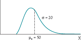
Figure A-1 Population distribution

Figure A-2 Sampling distribution of

Standard Probability Distributions

The normal distribution, discussed and shown in Figure A-2, is probably the most common probability distribution in statistics. Some other common distributions are the Poisson, a discrete distribution, and the negative exponential, a continuous distribution. In project management, the beta distribution plays an important role; a continuous distribution, it is generally skewed, as in Figure A-1. Two positive parameters, alpha and beta, determine the distribution's shape. Its mean, μ, and variance, σ², are given by

These are often approximated by

and the standard deviation approximated by

where

Recent research (Keefer and Verdini, 1993) has indicated that a much better approximation is given by

where

See Chapter 5 for another method for approximating μ and σ².

    BIBLIOGRAPHY

ANDERSON, D., D. SWEENEY, T. WILLIAMS, J. CAMM, and J. COCHRAN. Statistics for Business and Economics. 12th ed. Mason, OH: South-Western, 2014.

BHATTACHARYYA, G., and R. A. JOHNSON. Mathematical Statistics. Paramus, NJ: Prentice-Hall, 1999.

KEEFER, D. L., and W. A. VERDINI. “Better Estimation of PERT Activity Time Parameters.” Management Science, September 1993.

NETER, J., W. WASSERMAN, and G. A. WHITMORE. Applied Statistics, 4th ed. Boston: Allyn and Bacon, 1992.

WACKERLY, D., W. MENDENHALL, and R. L. SCHAEFFER. Mathematical Statistics with Applications, 7th ed. Belmont, CA: Thompson, 2008.