Streaming or online algorithms are useful as they don't require as much memory and processing power as other algorithms. This chapter has a recipe involving the calculation of statistical moments online (refer to Calculating the mean, variance, skewness, and kurtosis on the fly).

Also, in the Clustering streaming data with Spark recipe of Chapter 5, Web Mining, Databases, and Big Data, I covered another streaming algorithm.

Streaming algorithms are often approximate for fundamental reasons or because of roundoff errors. You should, therefore, try to use other algorithms if possible. Of course in many situations approximate results are good enough. For instance, it doesn't matter whether a user has 500 or 501 connections on a social media website. If you just send thousands of invitations, you will get there sooner or later.

Sketching is something you probably know from drawing. In that context, sketching means outlining rough contours of objects without any details. A similar concept exists in the world of streaming algorithms.

In this recipe, I cover the Count-min sketch (2003) by Graham Cormode and S. Muthu Muthukrishnan, which is useful in the context of ranking. For example, we may want to know the most viewed articles on a news website, trending topics, the ads with the most clicks, or the users with the most connections. The naive approach requires keeping counts for each item in a dictionary or a table. Dictionaries use hashing functions to calculate identifying integers, which serve as keys. For theoretical reasons, we can have collisions—this means that two or more items have the same key. The Count-min sketch is a two-dimensional tabular data structure that is small on purpose, and it uses hashing functions for each row. It is prone to collisions, leading to overcounting.

When an event occurs, for instance someone views an ad, we do the following:

Each event is clearly mapped to each row in the sketch. When we request the count, we follow the opposite path to obtain multiple counts. The lowest count gives an estimate for the count of this item.

The idea behind this setup is that frequent items are likely to dominate less common items. The probability of a popular item having collisions with unpopular items is larger than of collisions between popular items.

How to do it...

1. The imports are as follows:

   from nltk.corpus import brown
   from nltk.corpus import stopwords
   import dautil as dl
   from collections import defaultdict
   import matplotlib.pyplot as plt
   import numpy as np
   from IPython.display import HTML

2. Store the words of the NLTK Brown and stop words corpora in lists:

   words_dict = dl.collect.IdDict()
   dd = defaultdict(int)
   fid = brown.fileids(categories='news')[0]
   words = brown.words(fid)
   sw = set(stopwords.words('english'))

3. Count the occurrence of each stopword:

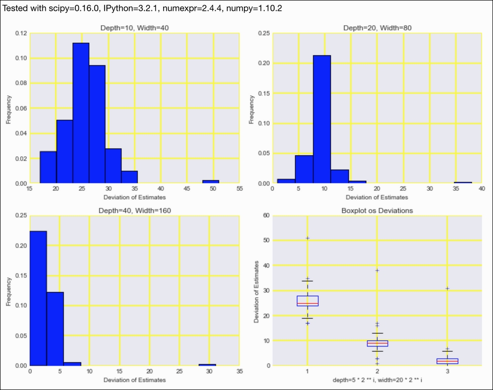
   for w in words:
       if w in sw:
           dd[w] += 1

4. Plot the distribution of count errors for various parameters of the Count-min sketch:

   sp = dl.plotting.Subplotter(2, 2, context)
   actual = np.array([dd[w] for w in sw])
   errors = []
   
   for i in range(1, 4):
       cm = dl.perf.CountMinSketch(depth=5 * 2 ** i,
                                   width=20 * 2 ** i)
   
       for w in words:
           cm.add(words_dict.add_or_get(w.lower()))
   
       estimates = np.array([cm.estimate_count(words_dict.add_or_get(w))
                           for w in sw])
       diff = estimates - actual
       errors.append(diff)
   
       if i > 1:
           sp.next_ax()
           
       sp.ax.hist(diff, normed=True,
               bins=dl.stats.sqrt_bins(actual))
       sp.label()
   
   sp.next_ax().boxplot(errors)
   sp.label()
   HTML(sp.exit())

Refer to the following screenshot for the end result:

The code is in the stream_demo.py file in this book's code bundle.