A lot of existing data is not labeled. It is still possible to learn from data without labels with unsupervised models. A typical task during exploratory data analysis is to find related items or clusters. We can imagine the Iris dataset, but without the labels:

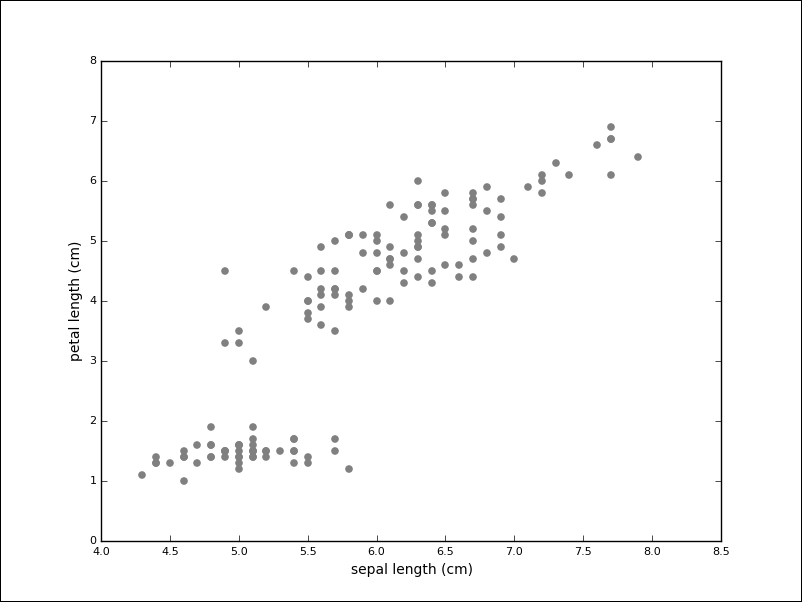
While the task seems much harder without labels, one group of measurements (in the lower-left) seems to stand apart. The goal of clustering algorithms is to identify these groups.

We will use K-Means clustering on the Iris dataset (without the labels). This algorithm expects the number of clusters to be specified in advance, which can be a disadvantage. K-Means will try to partition the dataset into groups, by minimizing the within-cluster sum of squares.

For example, we instantiate the KMeans model with n_clusters equal to 3:

>>> from sklearn.cluster import KMeans
>>> km = KMeans(n_clusters=3)

Similar to supervised algorithms, we can use the fit methods to train the model, but we only pass the data and not target labels:

>>> km.fit(iris.data)
KMeans(copy_x=True, init='k-means++', max_iter=300, n_clusters=3, n_init=10, n_jobs=1, precompute_distances='auto', random_state=None, tol=0.0001, verbose=0)

We already saw attributes ending with an underscore. In this case, the algorithm assigned a label to the training data, which can be inspected with the labels_ attribute:

>>> km.labels_
array([1, 1, 1, 1, 1, 1, ..., 0, 2, 0, 0, 2], dtype=int32)

We can already compare the result of these algorithms with our known target labels:

>>> iris.target
array([0, 0, 0, 0, 0, 0, ..., 2, 2, 2, 2, 2])

We quickly relabel the result to simplify the prediction error calculation:

>>> tr = {1: 0, 2: 1, 0: 2}
>>> predicted_labels = np.array([tr[i] for i in km.labels_])
>>> sum([p == t for (p, t) in zip(predicted_labels, iris.target)])
134

From 150 samples, K-Mean assigned the correct label to 134 samples, which is an accuracy of about 90 percent. The following plot shows the points of the algorithm predicted correctly in grey and the mislabeled points in red:

As another example for an unsupervised algorithm, we will take a look at Principal Component Analysis (PCA). The PCA aims to find the directions of the maximum variance in high-dimensional data. One goal is to reduce the number of dimensions by projecting a higher-dimensional space onto a lower-dimensional subspace while keeping most of the information.

The problem appears in various fields. You have collected many samples and each sample consists of hundreds or thousands of features. Not all the properties of the phenomenon at hand will be equally important. In our Iris dataset, we saw that the petal length alone seemed to be a good discriminator of the various species. PCA aims to find principal components that explain most of the variation in the data. If we sort our components accordingly (technically, we sort the eigenvectors of the covariance matrix by eigenvalue), we can keep the ones that explain most of the data and ignore the remaining ones, thereby reducing the dimensionality of the data.

It is simple to run PCA with scikit-learn. We will not go into the implementation details, but instead try to give you an intuition of PCA by running it on the Iris dataset, in order to give you yet another angle.

The process is similar to the ones we implemented so far. First, we instantiate our model; this time, the PCA from the decomposition submodule. We also import a standardization method, called StandardScaler, that will remove the mean from our data and scale to the unit variance. This step is a common requirement for many machine learning algorithms:

>>> from sklearn.decomposition import PCA
>>> from sklearn.preprocessing import StandardScaler

First, we instantiate our model with a parameter (which specifies the number of dimensions to reduce to), standardize our input, and run the fit_transform function that will take care of the mechanics of PCA:

>>> pca = PCA(n_components=2)
>>> X = StandardScaler().fit_transform(iris.data)
>>> Y = pca.fit_transform(X)

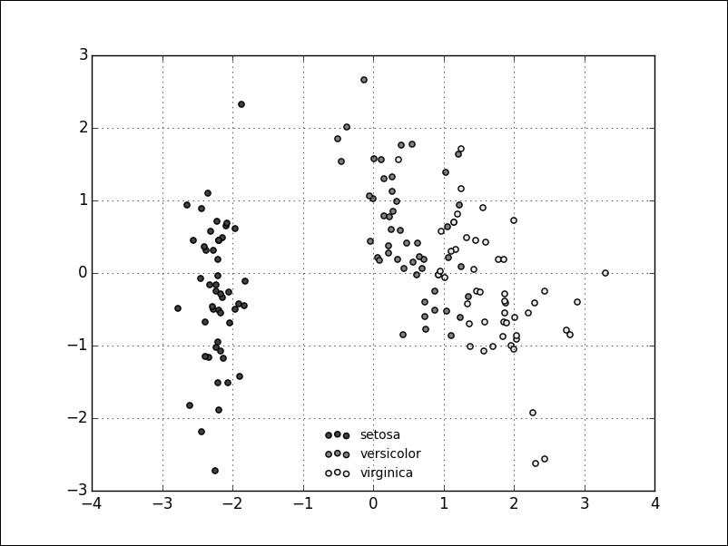
The result is a dimensionality reduction in the Iris dataset from four (sepal and petal width and length) to two dimensions. It is important to note that this projection is not onto the two existing dimensions, so our new dataset does not consist of, for example, only petal length and width. Instead, the two new dimensions will represent a mixture of the existing features.

The following scatter plot shows the transformed dataset; from a glance at the plot, it looks like we still kept the essence of our dataset, even though we halved the number of dimensions:

Dimensionality reduction is just one way to deal with high-dimensional datasets, which are sometimes effected by the so called curse of dimensionality.