Another useful method to visualize and make some of the initial analysis of the data is resampling, smoothing, and other rolling estimates. When resampling, a frequency keyword needs to be passed to the function. This is a combination of integers and letters, where the letters signify the type of the integer. To give you an idea, some of the frequency specifiers are as follows:

B, business, or D, calendar day

W, weekly

M, calendar month end or MS for start

Q, calendar quarter end or QS for start

A, calendar year end, or AS for start

H, hourly, T, minutely

Most of these can be modified by adding a B at the start of the specifier to change it to Business (month, quarter, year, and so on), and there are a few other keywords/descriptors that can be found in the Pandas documentation. Now let's try some of these out in the following examples. As this chapter contains several real-world data examples, which we use to highlight different things, feel free to play around with the data analysis. To resample the data by year, we simply pass an A to the resample() method:

temp.resample('A').head() 

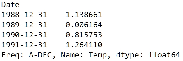
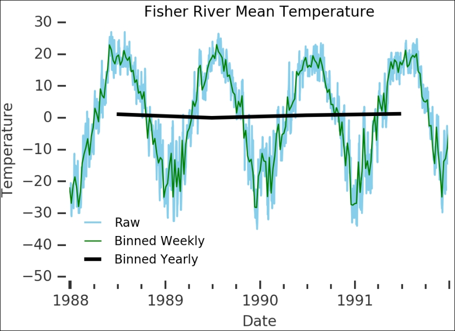
Here, the values are basically the mean of the year, with the label at the end of the year. Now let's make a plot with some of the resampling options to clearly show the variations that happen over these years.

First off, we plot the raw data, then we plot the data resampled to weekly basis, and lastly to yearly basis. However, if we give the frequency descriptor A on a yearly basis, it will simply be at the end of the year. It would be nice to show the year-to-year variation where the point is centered not in the beginning of the year but in the middle of the year. To accomplish this, we use the AS descriptor, giving us the data resampled over a year with the labels at the start, and then add an offset of roughly half a year with the loffset='178 D' keyword:

temp.plot(lw=1.5, color='SkyBlue') 
temp.resample('W').plot(lw=1, color='Green') 
temp.resample('AS', loffset='178 D').plot(color='k') 
plt.ylim(-50,30) 
plt.ylabel('Temperature') 
plt.title('Fisher River Mean Temperature') 
plt.legend(['Raw', 'Binned Weekly', 'Binned Yearly'], loc=3) 
despine(plt.gca()); 

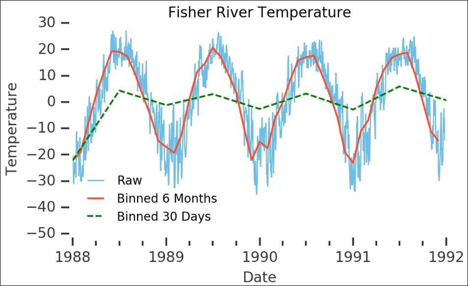
To make the legend more visible, I simply added some space with the plt.ylim() function. Now try to make a plot that looks like the following figure, with one month and six months resampling, plotted over the raw data:

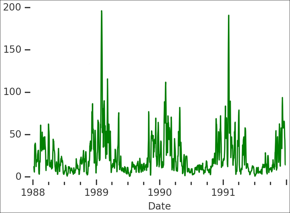
Sometimes we want to calculate a rolling value of something. While the resampling might look like a rolling mean, there is a specific function for it in Pandas. One of the things that we can do with this is combine the rolling mean over the time series and the minimum and maximum values in a region around it to highlight the variation to a nice figure. In the following figure, we plot the rolling mean in a window of 60, meaning that if the data is sampled in days, it will be 60 days. Furthermore, we have told the rolling mean to be centered in the window. To get the minimum and maximum from the raw data, we resample to months, take the minimum and maximum values, and fill the plot between them:

temp.plot(lw=1, alpha=0.5) 
pd.rolling_mean(temp, center=True, window=60).plot(color='Green') 
plt.fill_between(temp.resample('M', label='left',  
                               loffset='15 D').index, 
                 y1=temp.resample('M', how='max').values, 
                 y2=temp.resample('M', how='min').values, 
                 color='0.85') 
plt.gcf().autofmt_xdate() 
plt.ylabel('Temperature') 
despine(plt.gca()) 
plt.title('Fisher River Temperature'), 

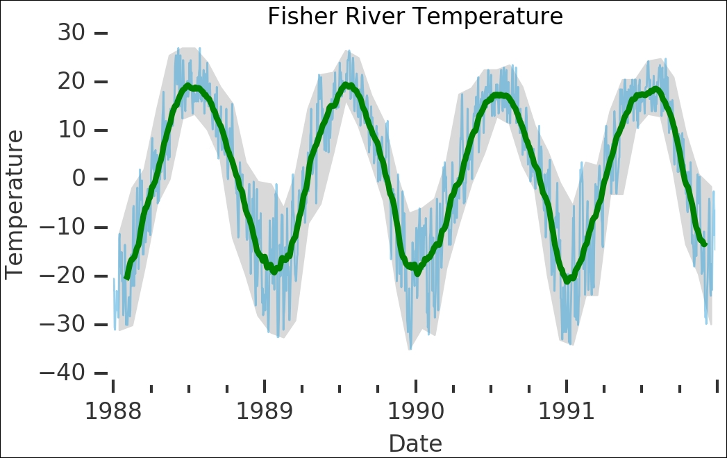
This already looks very good; the rolling mean reproduces the large-scale year-to-year variations of the temperature. While this is a kind of time series analysis and might be enough for first-order analysis and to get a handle of the data, we will look at some more complex methods to model variations. You can calculate other rolling values, such as the covariance:

pd.rolling_cov(temp, center=True, window=10).plot(color='Green') 
despine(plt.gca()); 

In this case, the covariance is in a window of 10 days and seems very high around the shift of the year. Another rolling value to calculate is the variance:

pd.rolling_var(temp, center=True, window=14).plot(color='Green') 
despine(plt.gca()); 

As we shall cover later on, analyzing the variance over time is very important for time series analysis. Try changing the window for both covariance and variance and see how they differ.

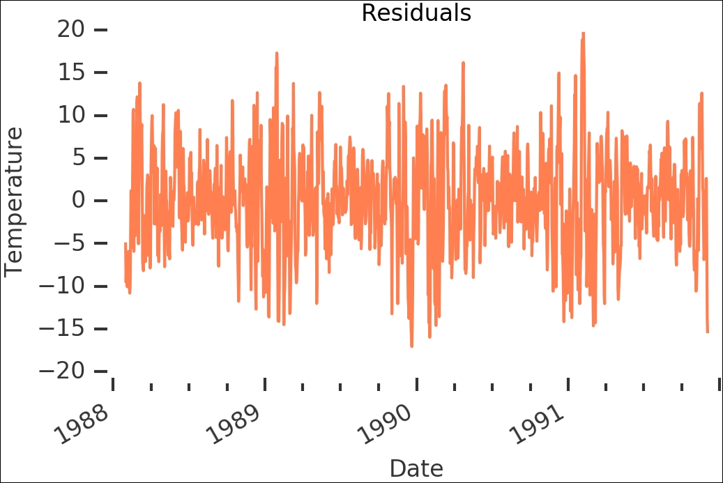
We calculated the rolling mean before and saw that it seems to follow the large-scale year-to-year variations of the data. Let's calculate the residuals to subtract this rolling mean from the raw data:

temp_residual = temp-pd.rolling_mean(temp, center=True, window=60) 

Visualizing the residuals, we can see that there is still some periodicity in it. To analyze a time series, we need the data to contain as few of these large-scale patterns as possible:

temp_residual.plot(lw=1.5, color='Coral') 
despine(plt.gca()) 
plt.gcf().autofmt_xdate() 
plt.title('Residuals') 
plt.ylabel('Temperature'), 

Time series analysis is mostly based on the fact that the current value might depend on only a few of the previous values and to a varying extent. So to analyze the data, we need to get rid of these. This naturally leads us to the next topic—stationarity. In the next section, we will discuss this, show you how to test if your data is stationary, and a couple of ways to make it stationary if it is not.