
Seaborn color palettes are similar to matplotlib colormaps. Color can help you discover patterns in data and is an important visualization component. Seaborn has a wide range of color palettes, which I will try to visualize in this recipe.
- The imports are as follows:
import seaborn as sns
import matplotlib.pyplot as plt
import matplotlib as mpl
import numpy as np
from dautil import plotting
- Use the following function that helps plot the palettes:
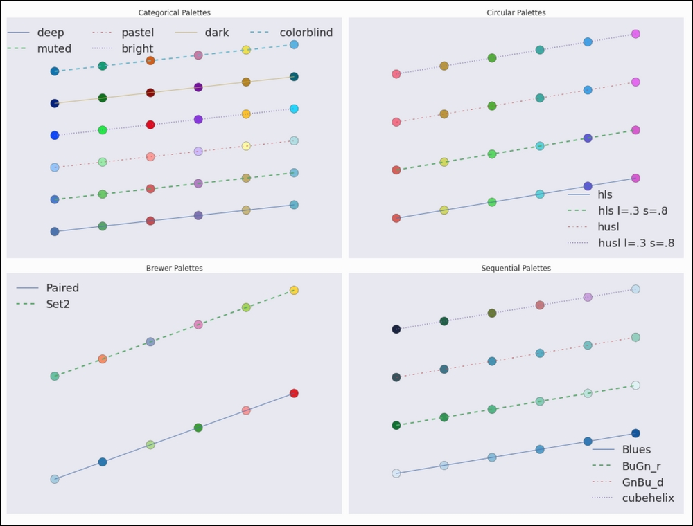
def plot_palette(ax, plotter, pal, i, label, ncol=1): n = len(pal) x = np.linspace(0.0, 1.0, n) y = np.arange(n) + i * n ax.scatter(x, y, c=x, cmap=mpl.colors.ListedColormap(list(pal)), s=200) plotter.plot(x,y, label=label) handles, labels = ax.get_legend_handles_labels() ax.legend(loc='best', ncol=ncol, fontsize=18) - Categorical palettes are useful for categorical data, for instance, gender or blood type. The following function plots some of the Seaborn categorical palettes:
def plot_categorical_palettes(ax): palettes = ['deep', 'muted', 'pastel', 'bright', 'dark', 'colorblind'] plotter = plotting.CyclePlotter(ax) ax.set_title('Categorical Palettes') for i, p in enumerate(palettes): pal = sns.color_palette(p) plot_palette(ax, plotter, pal, i, p, 4) - Circular color systems usually use HLS (Hue Lightness Saturation) instead of RGB (red green blue) color spaces. They are useful if you have many categories. The following function plots palettes using HSL systems:
def plot_circular_palettes(ax): ax.set_title('Circular Palettes') plotter = plotting.CyclePlotter(ax) pal = sns.color_palette("hls", 6) plot_palette(ax, plotter, pal, 0, 'hls') sns.hls_palette(6, l=.3, s=.8) plot_palette(ax, plotter, pal, 1, 'hls l=.3 s=.8') pal = sns.color_palette("husl", 6) plot_palette(ax, plotter, pal, 2, 'husl') sns.husl_palette(6, l=.3, s=.8) plot_palette(ax, plotter, pal, 3, 'husl l=.3 s=.8') - Seaborn also has palettes, which are based on the online ColorBrewer tool (http://colorbrewer2.org/). Plot them as follows:
def plot_brewer_palettes(ax): ax.set_title('Brewer Palettes') plotter = plotting.CyclePlotter(ax) pal = sns.color_palette("Paired") plot_palette(ax, plotter, pal, 0, 'Paired') pal = sns.color_palette("Set2", 6) plot_palette(ax, plotter, pal, 1, 'Set2') - Sequential palettes are useful for wide ranging data, for instance, differing by orders of magnitude. Use the following function to plot them:
def plot_sequential_palettes(ax): ax.set_title('Sequential Palettes') plotter = plotting.CyclePlotter(ax) pal = sns.color_palette("Blues") plot_palette(ax, plotter, pal, 0, 'Blues') pal = sns.color_palette("BuGn_r") plot_palette(ax, plotter, pal, 1, 'BuGn_r') pal = sns.color_palette("GnBu_d") plot_palette(ax, plotter, pal, 2, 'GnBu_d') pal = sns.color_palette("cubehelix", 6) plot_palette(ax, plotter, pal, 3, 'cubehelix') - The following lines call the functions we defined:
%matplotlib inline

fig, axes = plt.subplots(2, 2, figsize=(16, 12))
plot_categorical_palettes(axes[0][0])
plot_circular_palettes(axes[0][1])
plot_brewer_palettes(axes[1][0])
plot_sequential_palettes(axes[1][1])
plotting.hide_axes(axes)
plt.tight_layout()
The complete code is available in the choosing_palettes.ipynb file in this book's code bundle. Refer to the following plot for the end result:
- The seaborn color palettes documentation at https://web.stanford.edu/~mwaskom/software/seaborn/tutorial/color_palettes.html (retrieved July 2015)
..................Content has been hidden....................
You can't read the all page of ebook, please click here login for view all page.