In this section, we will show short examples for both classification and regression.

Classification problems are pervasive: document categorization, fraud detection, market segmentation in business intelligence, and protein function prediction in bioinformatics.

While it might be possible for hand-craft rules to assign a category or label to new data, it is faster to use algorithms to learn and generalize from the existing data.

We will continue with the Iris dataset. Before we apply a learning algorithm, we want to get an intuition of the data by looking at some values and plots.

All measurements share the same dimension, which helps to visualize the variance in various boxplots:

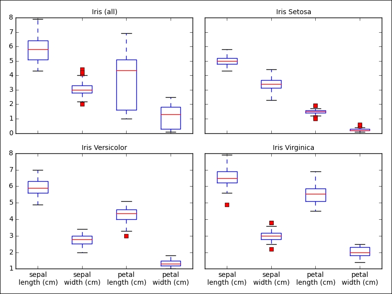
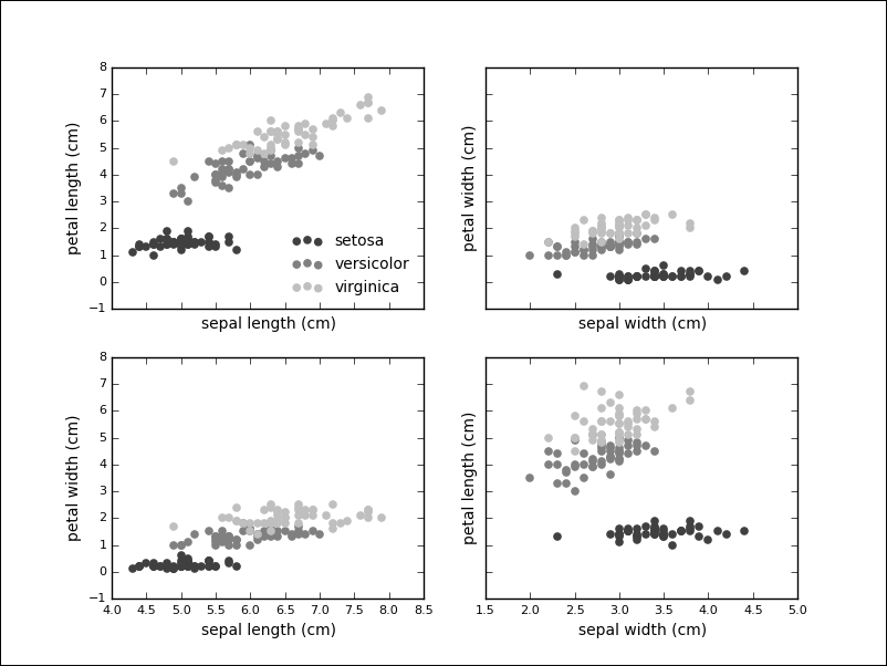
We see that the petal length (the third feature) exhibits the biggest variance, which could indicate the importance of this feature during classification. It is also insightful to plot the data points in two dimensions, using one feature for each axis. Also, indeed, our previous observation reinforced that the petal length might be a good indicator to tell apart the various species. The Iris setosa also seems to be more easily separable than the other two species:

From the visualizations, we get an intuition of the solution to our problem. We will use a supervised method called a Support Vector Machine (SVM) to learn about a classifier for the Iris data. The API separates models and data, therefore, the first step is to instantiate the model. In this case, we pass an optional keyword parameter to be able to query the model for probabilities later:

>>> from sklearn.svm import SVC
>>> clf = SVC(probability=True)

The next step is to fit the model according to our training data:

>>> clf.fit(iris.data, iris.target)
SVC(C=1.0, cache_size=200, class_weight=None, coef0=0.0,
    degree=3, gamma=0.0, kernel='rbf', max_iter=-1,
    probability=True, random_state=None, shrinking=True,
    tol=0.001, verbose=False)

With this one line, we have trained our first machine learning model on a dataset. This model can now be used to predict the species of unknown data. If given some measurement that we have never seen before, we can use the predict method on the model:

>>> unseen = [6.0, 2.0, 3.0, 2.0]
>>> clf.predict(unseen)
array([1])
>>> iris.target_names[clf.predict(unseen)]
array(['versicolor'],
      dtype='|S10')

We see that the classifier has given the versicolor label to the measurement. If we visualize the unknown point in our plots, we see that this seems like a sensible prediction:

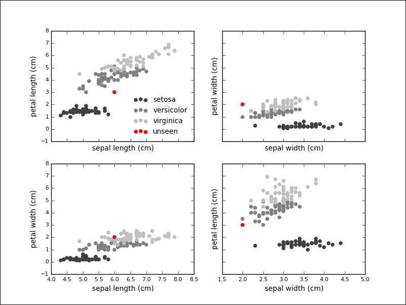
In fact, the classifier is relatively sure about this label, which we can inquire into by using the predict_proba method on the classifier:

>>> clf.predict_proba(unseen)
array([[ 0.03314121,  0.90920125,  0.05765754]])

Our example consisted of four features, but many problems deal with higher-dimensional datasets and many algorithms work fine on these datasets as well.

We want to show another algorithm for supervised learning problems: linear regression. In linear regression, we try to predict one or more continuous output variables, called regress ands, given a D-dimensional input vector. Regression means that the output is continuous. It is called linear since the output will be modeled with a linear function of the parameters.

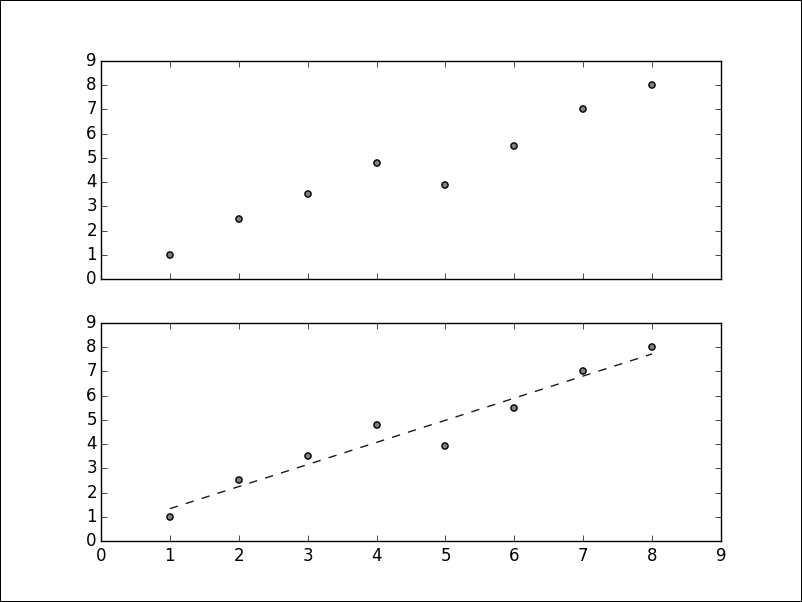
We first create a sample dataset as follows:

>>> import matplotlib.pyplot as plt
>>> X = [[1], [2], [3], [4], [5], [6], [7], [8]]
>>> y = [1, 2.5, 3.5, 4.8, 3.9, 5.5, 7, 8]
>>> plt.scatter(X, y, c='0.25')
>>> plt.show()

Given this data, we want to learn a linear function that approximates the data and minimizes the prediction error, which is defined as the sum of squares between the observed and predicted responses:

>>> from sklearn.linear_model import LinearRegression
>>> clf = LinearRegression()
>>> clf.fit(X, y)

Many models will learn parameters during training. These parameters are marked with a single underscore at the end of the attribute name. In this model, the coef_ attribute will hold the estimated coefficients for the linear regression problem:

>>> clf.coef_
array([ 0.91190476])

We can plot the prediction over our data as well:

>>> plt.plot(X, clf.predict(X), '--', color='0.10', linewidth=1)

The output of the plot is as follows:

The above graph is a simple example with artificial data, but linear regression has a wide range of applications. If given the characteristics of real estate objects, we can learn to predict prices. If given the features of the galaxies, such as size, color, or brightness, it is possible to predict their distance. If given the data about household income and education level of parents, we can say something about the grades of their children.

There are numerous applications of linear regression everywhere, where one or more independent variables might be connected to one or more dependent variables.