We present another method of investigating the leverage effect (fact 5). To do so, we use the VIX (CBOE Volatility Index), which is a popular metric of the stock market's expectation regarding volatility. The measure is implied by option prices on the S&P 500 index. We take the following steps:

1. Download and preprocess the prices of the S&P 500 and VIX:

df = yf.download(['^GSPC', '^VIX'], 
                 start='1985-01-01', 
                 end='2018-12-31',
                 progress=False)
df = df[['Adj Close']]
df.columns = df.columns.droplevel(0)
df = df.rename(columns={'^GSPC': 'sp500', '^VIX': 'vix'})

2. Calculate the log returns (we can just as well use percentage change-simple returns):

df['log_rtn'] = np.log(df.sp500 / df.sp500.shift(1))
df['vol_rtn'] = np.log(df.vix / df.vix.shift(1))
df.dropna(how='any', axis=0, inplace=True)

3. Plot a scatterplot with the returns on the axes and fit a regression line to identify the trend:

corr_coeff = df.log_rtn.corr(df.vol_rtn)

ax = sns.regplot(x='log_rtn', y='vol_rtn', data=df, 
                 line_kws={'color': 'red'})
ax.set(title=f'S&P 500 vs. VIX ($\rho$ = {corr_coeff:.2f})',
       ylabel='VIX log returns',
       xlabel='S&P 500 log returns')

We additionally calculated the correlation coefficient between the two series and included it in the title:

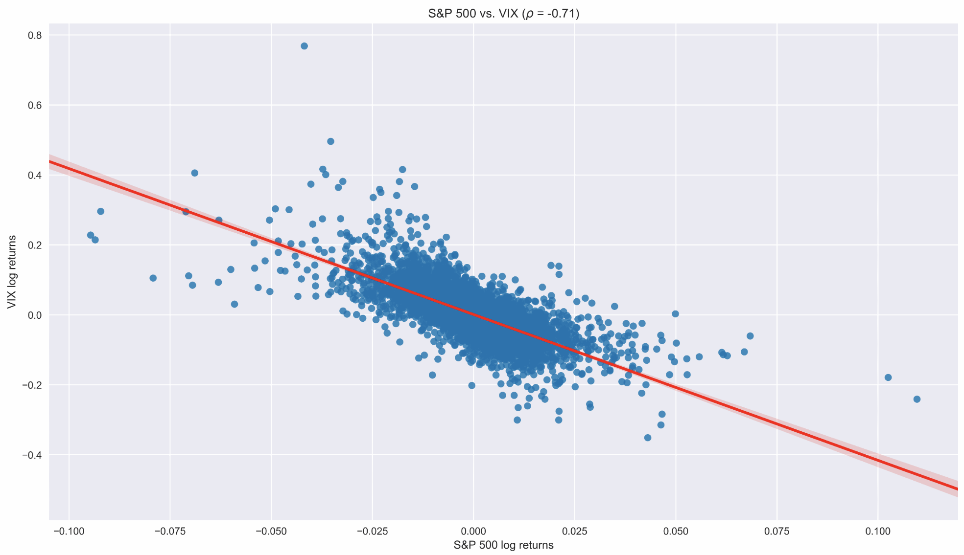
We can see that both the negative slope of the regression line and a strong negative correlation between the two series confirm the existence of the leverage effect in the return series.