
Circular Buffering
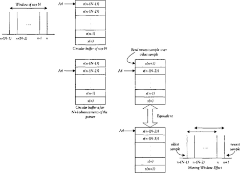
In many DSP algorithms, such as filtering, adaptive filtering, or spectral analysis, we need to shift data or update samples (i.e., we need to deal with a moving window). The direct method of shifting data is inefficient and uses many cycles. Circular buffering is an addressing mode by which a moving-window effect can be created without the overhead associated with data shifting. In a circular buffer, if a pointer pointing to the last element of the buffer is incremented, it is automatically wrapped around and pointed back to the first element of the buffer. This provides an easy mechanism to exclude the oldest sample while including the newest sample, creating a moving-window effect as illustrated in Figure 8-1.
Some DSPs have dedicated hardware for doing this type of addressing. On the C6x processor, the arithmetic logic unit has the circular addressing mode capability built into it. To use circular buffering, first the circular buffer sizes need to be written into the BK0 and BK1 block size fields of the Address Mode Register (AMR), as shown in Figure 8-2. The C6x allows two independent circular buffers of powers of 2 in size. Buffer size is specified as 2(N+1) bytes, where N indicates the value written to the BK0 and BK1 block size fields.
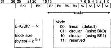
Then, the register to be used as the circular buffer pointer needs to be specified by setting appropriate bits of AMR to 1. For example, as shown in Figure 8-2, for using A4 as a circular buffer pointer, bit 0 or 1 is set to 1. Of the 32 registers on the C6x, 8 can be used as circular buffer pointers: A4 through A7 and B4 through B7. Note that linear addressing is the default mode of addressing for these registers.
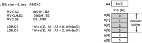
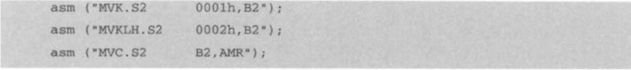
Figure 8-3 shows the code to set up the AMR register for a circular buffer of size 8, together with a load example. To set up such a circular buffer in C, one must use so-called in-line assembly as follows:
When using circular buffers, care must be taken to align data on the buffer size boundary. In C, this can be achieved by using pragma directives. Pragma directives indicate what kinds of preprocessing are done by the compiler. The DATA_ALIGN pragma can be used to align symbol to a power of 2 alignment boundary constant (in bytes) as follows:
![]()
Lab. 5 Adaptive Filtering
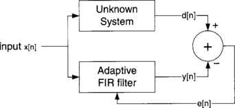
Adaptive filtering is used in many applications ranging from noise cancellation to system identification. In most cases, the coefficients of an FIR filter are modified according to an error signal in order to adapt to a desired signal. In this lab, a system identification example is implemented wherein an adaptive FIR filter is used to adapt to the output of a seventh-order IIR bandpass filter. The IIR filter is designed in MATLAB and implemented in C. The adaptive FIR is first implemented in C and later in assembly using circular buffering.
In system identification, the behavior of an unknown system is modeled by accessing its input and output. An adaptive FIR filter can be used to adapt to the output of the system based on the same input. The difference in the output of the system, d[n], and the output of the adaptive filter, y[n], constitutes the error term e[n], which is used to update the coefficients of the FIR filter. Figure 8-4 illustrates this process.
The error term calculated from the difference of the outputs of the two systems is used to update each coefficient of the FIR filter according to the formula (least mean square (LMS) algorithm [1]):
where the h‘s denote the unit sample response or FIR filter coefficients. The output y[n] is required to approach d[n]. The term δ indicates step size. A small step size will ensure convergence, but results in a slow adaptation rate. A large step size, though faster, may lead to skipping over the solution.
L5.1 Design of IIR Filter
A seventh-order bandpass IIR filter is used to act as the unknown system. The adaptive FIR is designed to adapt to the response of the IIR system. Considering a sampling frequency of 8 kHz, let the IIR filter have a passband from π/3 to 2π/3 (radians), with a stopband attenuation of 20dB. The design of the filter can be easily achieved with the MATLAB function ‘yulewalk’ [2]. The following MATLAB code may be used to obtain the coefficients of the filter:
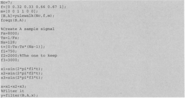
It can be verified that the filter is working by deploying a simple composite signal. Using the MATLAB function ‘filter’, verify the design by observing that the frequency components of the composite signal falling in the stopband are removed. (See Figure 8-5 and Table 8-1.)

L5.2 IIR Filter Implementation
The implementation of the IIR filter is first done in C, using the following difference equation
where ak‘s and bk‘s denote the IIR filter coefficients. Two arrays are required, one for the input samples x[n] and the other for the output samples y[n]. Given that the filter is of the order 7, an input array of size 8 and an output array of size 7 are considered. The arrays are used to simulate a circular buffer, since in C this property of the CPU cannot be accessed. As a new sample comes in, all elements in the input array are shifted down by one. In this manner, the last element is lost and the last eight samples are always kept. The input array is used to calculate the resulting output, and then the output is used to modify the output array. A simple implementation of this scheme is shown in the following code, which is a modification of the sampling program in Lab 2:

By running this program while connecting a function generator and an oscilloscope to the line-in and line-out of the audio daughter card, the functionality of the IIR filter can be verified. Whenever the DRR receives a new incoming sample from the function generator, the ISR is invoked. Then, the new sample is right shifted by the scaling factor S. This factor is included for the correction of any possible overflow. In this lab, there is no need for shifting. Once the new sample is scaled, the last eight samples are kept by discarding the oldest sample and adding the new sample to the input buffer IIRwindow. This operation is done by shifting the data in the input array. Note that this array is global and is initialized to zero in the main function.
Now that the last eight samples are ready to be used, it is time to compute BSUM (b coefficient terms) and ASUM (a coefficient terms). Attention needs to be paid to the datatype of BSUM, ASUM, the coefficient arrays, and the input array. The datatype of the coefficient arrays is short, so the coefficients are converted to Q-15 format by multiplying them by 0x7FFF in the main function. The datatype of the input array IIRwindow is also short. However, the datatype of ASUM or BSUM is int (32 bits). Therefore, ASUM and BSUM need to be left shifted by 1 to eliminate the extended sign bit, since the multiplication of Q-15 by Q-15 results in Q-30 representation. In order to obtain the IIR output IIR_OUT, the partial output ASUM is subtracted from BSUM. Note that the difference (BSUM – ASUM) is right shifted by 16 to convert it to a short datatype. The IIR output is then used to compute ASUM in the next iteration. Finally, the IIR output is scaled back and sent to the data transmit register (DXR).
L5.3 Adaptive FIR Filter
By replacing the following piece of code with MCBSP_write (hMcbsp, IIR_OUT≥S) in the previous IIR function, we can make a FIR filter to adapt to the output of the IIR filter:
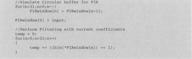
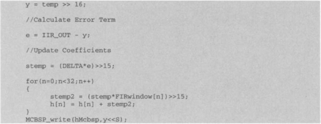
In this program, a 32-coefficient FIR filter is used to adapt to the output of the IIR filter. To do this in C, an additional buffer of length 32 is needed: one for the input buffer FIRwindow and the other for the coefficients h of the FIR filter. Initially all the data in both arrays are zero. The order of processing is as follows: First, the last 32 samples are shifted. The shift discards the oldest sample and adds the newly read sample into the input buffer. Next, the FIR filtering is done by performing a dot-product between the coefficients h and the input buffer. The dot- product is converted to Q-15 format by left shifting it by 1. Then, the error term between the IIR and the FIR filter output is computed. The coefficients of the FIR filter are updated to match the IIR and FIR filter outputs. Finally, the FIR filter output is sent to the DXR. By using a function generator and an oscilloscope, the adaptation process can be observed by scanning through different frequencies.
It is worth mentioning a point about the step size δ. In a floating-point processor, δ is usually chosen to be in the range of e−7. However, the precision on the fixed-point C6x does not allow for such a small number. We can at most use 0x0001, which is 1/(215) ≈ 0.0000305. When a multiplication is done with this number, any positive number will be defaulted to 0 and any negative number to −1. This is due to the nature of multiplication of Q-15 format numbers, where the product is right shifted by 15. However, the contribution of negative numbers to the coefficients is sufficient for the LMS algorithm to converge. Using a larger δ for this adaptive filtering example results in faster adaptation, but convergence is not guaranteed. Satisfactory results can be observed with δ in the range of 0x0100 to 0x0001.
The reason for implementing the LMS algorithm in assembly is to make use of the circular buffering capability of the C6x. Of the 32 registers on the C6x, 8 can perform circular addressing. These registers are A4 through A7 and B4 through B7. Since linear addressing is the default mode of addressing, each of these registers must be specified as circular using the AMR register. The lower 16 bits of the AMR register are used to select the mode for each of the 8 registers. The upper 10 bits (6 are reserved) are used to set the length of the circular buffer. Buffer size is determined by 2(N+1) bytes, where N is the value appearing in the block size fields of the AMR register.
Since we are using both C and assembly, we have to initialize the circular buffer when we enter the assembly part of the program. During the execution of the assembly code, the register used in the circular mode allows a certain location in memory to always contain the newest sample. As the assembly code is completed and returns to the calling C program, the location of the pointer to the buffer must be saved and the AMR register must be returned to the linear mode, since leaving it in the circular mode disrupts the flow of the program.
To do such a task, a section of memory not used by the compiler must be set aside for the buffer, and the coefficients. A simple way to do this is to reserve 64 bytes for the coefficients, 64 bytes for the buffer, and 4 bytes for the pointer. Since the data and coefficients are short formatted here, 64 bytes are used to provide 32 locations. The following memory representation is employed for this purpose:
| 0x00000200 | 64 Bytes, Circular Buffer |
| 0x00000240 | 64 Bytes, Coefficients |
| 0x00000280 | 4 Bytes, Pointer |
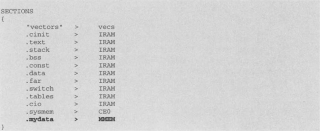
The command file must also be modified. A simple assembly file is needed to initialize the memory locations with zeros. The following command file defines a new memory section called mmem in the internal memory and uses it for the code section .mydata:

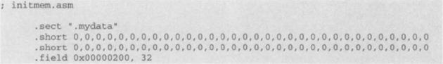
The file initmem.asm appearing next is used to initialize the memory locations with zeros and set the pointer to the first free location, which is 0x00000200:
With the command file and the brief assembly code just shown, it is ensured that 132 bytes of space starting at 0x00000200, will not be used for anything other than the adaptive filter. Now, as mentioned before, the circular buffer must be initialized upon entering the assembly part. To do this, it is necessary to modify the AMR register. Since a buffer of length 32 is needed, one must have 5 in the block fields (block size = 2(5+1) = 64). With register A5 as the circular buffer pointer, the value to set the AMR register becomes 0x00050004. Entering the assembly function, the last pointer location is read from 0x00000280. The last free location of the buffer is saved to the same location upon exit. The following code shows how this is achieved:
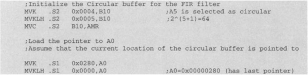
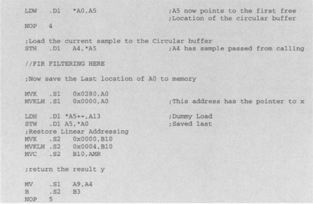
Upon entering the assembly function, the AMR register is loaded with 0x00050004 for the desired circular buffer operation. Then, the memory location (or address) to which register A5 was last pointing is loaded into A5. Hence, A5 points to the first free location of the circular buffer, and the content of register A4 (the newest sample passed from the C program) is stored in this location. After adaptive filtering, the address pointed to by A5 is stored at the location 0x00000280. Note that here a dummy load is performed to increment the pointer so that it points to the last element (the next free location). This is needed because only a load or store operation increments the pointer in a circular fashion.
The following adaptive FIR filter assembly code resides in the section of the foregoing code labeled ‘FIR FILTERING HERE’:
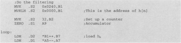

In this code, the adaptive filtering process is done via two separate loops. The first loop calculates a dot-product between the coefficients and the samples. The error term is then calculated and used in the second loop for updating the coefficients, based on the input samples. Notice that a circular buffer is not used for the coefficients, since they do not change in a time-windowed manner, as do the input samples.
We now have two versions of the adaptive filter. One is written entirely in C, and the other is a mix of C and assembly. When the entire C program runs in the external memory, the output does not adapt to the IIR filter output. Only when the entire C program runs in the internal memory does the output adapt to the IIR filter output. Also, when the assembly part of the mixed C/assembly program runs in the external memory, the output adapts to the IIR filter output. Of course, the assembly part of the program can be configured to run in the internal memory space, where the number of cycles is noticeably reduced. The main reason for running the C code from the internal memory space is that running it from the external memory is too slow and samples get missed. Table 8-2 gives a summary of the timing cycles for different memory options of the adaptive filtering program. All the programs associated with this lab are placed on the accompanying CD-ROM.