
Code Optimization
Four relatively simple modifications of assembly code can be done to generate a more efficient code. These modifications make use of the available C6x resources such as multiple buses, functional units, pipelined CPU, and memory organization. They include (a) using parallel instructions, (b) eliminating delays or NOPs, (c) unrolling loops, and (d) using word-wide data.
Wherever possible, parallel instructions should be used to make maximum use of idle functional units. It should be noted that, whenever the order in which instructions appear is important, care must be taken not to have any dependency in the operands of the instructions within a parallel instruction.
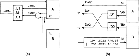
It may become necessary to have cross paths when making instructions parallel. There are two types of cross paths: data and address. As illustrated in Figure 7-1 (a), in data cross paths, one source part of an instruction on the A or B side comes from the other side. A cross path is indicated by x as part of functional unit assignment. The destination is determined by the unit index 1 or 2. As an example, we might have:
![]()
In address cross paths, a .D unit gets its data address from the address bus on the other side. There are two address buses: DA1 and DA2, also known as T1 and T2, respectively. Figure 7-1 (b) illustrates an example where a load and a store are done in parallel via the address cross paths.
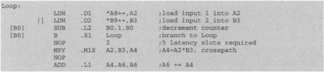
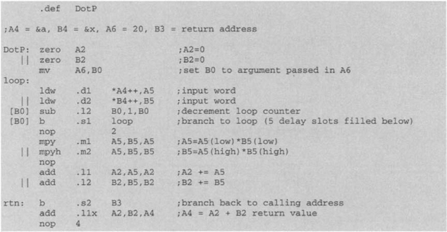
Wherever possible, branches should be placed five places ahead of where they are intended to appear. This would create a delayed branch, minimizing the number of NOPs. This approach should also be applied to load and multiply instructions that involve four delays and one delay, respectively. If the code size is of no concern, loops should be repeated or copied. By copying or unrolling a loop, fewer clock cycles would be needed, primarily due to deleting branches. Figure 7-2 shows the optimized version of the dot-product loop incorporating the preceding steps.
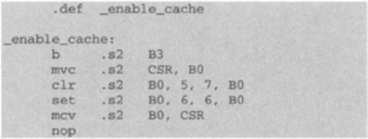
Considering that there exists a delay associated with getting information from off-chip memory, program codes should be run from the on-chip RAM whenever possible. In situations where program codes would not fit into the on-chip RAM, faster execution can be achieved by placing the most time-consuming routine or function in the on-chip memory. The C6x has a cache feature which can be enabled to turn the program RAM into cache memory. This is done by setting the program cache control (PCC) bits of the CSR to 010. For repetitive operations or loops, it is recommended that this feature is enabled, since there is then a good chance the cache will contain the needed fetch packet and the EMIF will be unused, speeding up code execution. Figure 7-3 shows the code for enabling the cache feature. The instruction CLR and SET are used to clear and set bits from the second argument position to the third argument position. For more detailed operation of cache and its options, refer to the CPU Reference Guide [1].
7.1 Word-Wide Optimization
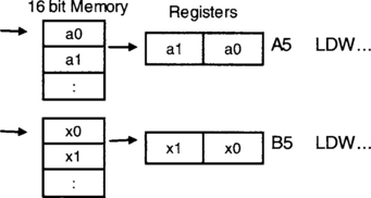
If data are in halfwords (16 bits), it is possible to perform two loads in one instruction, since the CPU registers are 32 bits wide. In other words, as shown in Figure 7-4, one data can get loaded into the lower part of a register and another one into the upper part.
This way, to do multiplication, two multiplication instructions MPY and MPYH, should be used, one taking care of the lower part and the other of the upper part, as shown in Figure 7-5. Note that A5 and B5 appear as arguments in both MPY and MPYH instructions. This does not pose any conflict, since, on the C6x, up to four reads of a register in one cycle are allowed.
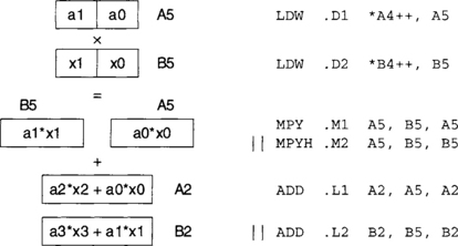
Figure 7-6 provides the word-wide optimized version of the dot-product function DotP ( ). When the looping is finished, register A2 would contain the sum of even terms and register B2 the sum of odd terms. To obtain the total sum, these registers are added outside the loop.
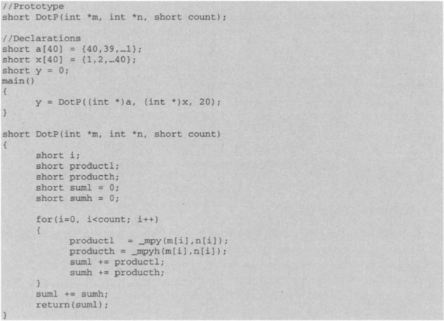
Out of the preceding modifications, it is possible to do the last one, word-wide optimization, in C. This demands using an appropriate datatype in C. Figure 7-7 shows the word-wide optimized C code by using the _mpy ( ) and _mpyh ( ) intrinsics.
7.2 Mixing C and Assembly
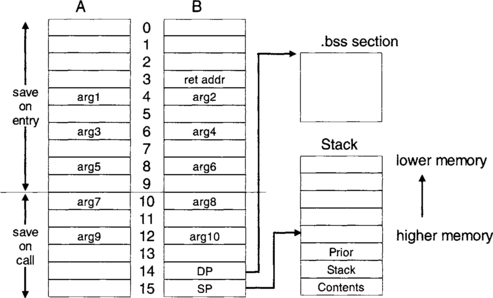
To mix C and assembly, it is necessary to know the register convention used by the compiler to pass arguments. This convention is illustrated in Figure 7-8. DP, the base pointer, points to the beginning of the .bss section, containing all global and static variables. SP, the stack pointer, points to local variables. The stack grows from higher memory to lower memory, as indicated in Figure 7-8. The space between even registers (odd registers) is used when passing 40-bit or 64-bit values.
7.3 Software Pipelining
Software pipelining is a technique for writing highly efficient assembly loop codes on the C6x processor. Using this technique, all functional units on the processor are fully utilized within one cycle. However, to write hand-coded software pipelined assembly code, a fair amount of coding effort is required, due to the complexity and number of steps involved in writing such code. In particular, for complex algorithms encountered in many communications, and signal/image processing applications, hand-coded software pipelining considerably increases coding time. The C compiler at the optimization levels 2 and 3 (-o2 and –o3) performs software pipelining to some degree. (See Figure 4-1.) Compared with linear assembly, the increase in code efficiency when writing hand-coded software pipelining is relatively slight.
7.3.1 Linear Assembly
Linear assembly is a coding scheme that allows one to write efficient codes (compared with C) with less coding effort (compared with hand-coded software pipelined assembly). The assembly optimizer is the software tool that parallelizes linear assembly code across the eight functional units. It attempts to achieve a good compromise between code efficiency and coding effort.
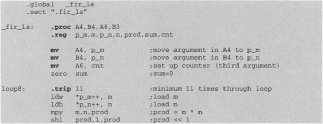
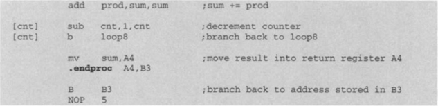
In a linear assembly code, it is not required to specify any functional units, registers, and NOP’s. Figure 7-9 shows the linear assembly code version of the dot-product function. The directives .proc and .endproc define the beginning and end, respectively, of the linear assembly procedure. The symbolic names p_m, p_n, m, n, count, prod, and sum are defined by the .reg directive. The names p_m, p_n, and count are associated with the registers A4, B4, and A6 by using the assignment MV instruction.
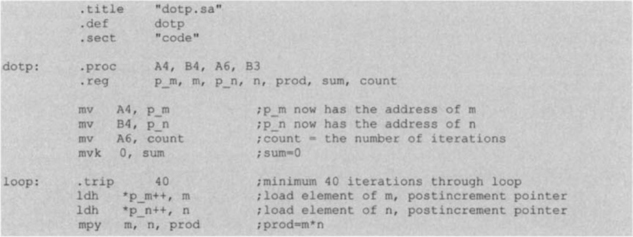
As per the register convention, the arguments are passed into and out of the procedure via registers A4, B4, A6, and B3. A4 is used to pass the address of m (argl), B4 the address of n (arg2), and A6 the address of sum (arg3). Register B3, referred to as a preserved register, is passed in and out with no modification. This is done to prevent it from being used by the procedure. Here, this register is used to contain the return address reached by the branch instruction outside of the procedure. Preserved registers must be specified in both input and output arguments while not being used within the procedure. Table 7-1 provides a list of linear assembly directives.
Table 7-1
| Directive | Description | Restrictions |
| .call | Calls a function | Valid only within procedures |
| .cproc | Start a C/C++ callable procedure | Must use with. endproc |
| .endproc | End a C/C++ callable procedure | Must use with. cproc |
| .endproc | End a procedure | Must use with. proc; cannot use variables in the register parameter |
| .mdep | Indicates a memory dependence | Valid only within procedures |
| .mptr | Avoid memory bank conflicts | Valid only within procedures; can use variables in the register parameter |
| .no_mdep | No memory aliases in the function | Valid only within procedures |
| .proc | Start a procedure | Must use with. endproc; cannot use variables in the register parameter |
| .reg | Declare variables | Valid only within procedures |
| .reserve | Reserve register use | |
| .return | Return value to procedure | Valid only within. cproc procedures |
| .trip | Specify trip count value | Valid only within procedures |
If the number of iterations is known, a .trip directive should be used for the assembler optimizer to generate the pipelined code. For n iterations of a loop, in a pipelined code, the loop is repeated n’ times, where n’ = n – prolog length (prolog will be explained later in the chapter). The number of iterations, n’, is known as the minimum trip count. If .trip is greater than or equal to n’, only the pipelined code is created. Otherwise, both the pipelined and the non-pipelined code are created. If .trip is not specified, only the non-pipelined code is created. In C, the function _n_assert ( ) is used to provide the same information as .trip.
To further optimize a linear assembly code, partitioning information can be added. Such information consist of the assignment of data paths to instructions.
7.3.2 Hand-Coded Software Pipelining
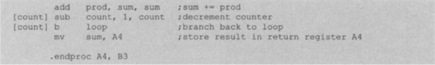
First let us review the pipeline concept. Figures 7-10(b) and 7-10(c) show a non-pipelined and a pipelined version of the loop code shown in Figure 7-10(a). As can be seen from this figure, the functional units in the non-pipelined version are not fully utilized, leading to more cycles compared with the pipelined version. There are three stages to a pipelined code, named prolog, loop kernel, and epilog. Prolog corresponds to instructions that are needed to build up a loop kernel or loop cycle, and epilog to instructions that are needed to complete all loop iterations. When a loop kernel is established, the entire loop is done in one cycle via one parallel instruction using the maximum number of functional units. This parallelism is what causes a reduction in the number of cycles.
Three steps are needed to produce a hand-coded software pipelined code from a linear assembly loop code: (a) drawing a dependency graph, (b) setting up a scheduling table, and (c) deriving the pipelined code from the scheduling table.
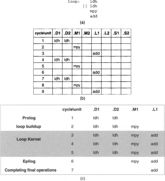
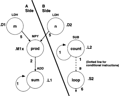
In a dependency graph (see Figure 7-11 for the terminology), the nodes denote instructions and symbolic variable names. The paths show the flow of data and are annotated with the latencies of their parent nodes. To draw a dependency graph for the loop part of the dot-product code, we start by drawing nodes for the instructions and symbolic variable names.
After the basic dependency graph is drawn, a functional unit is assigned to each node or instruction. Then, a line is drawn to split the workload between the A- and B-side data paths as equally as possible. It is apparent that one load should be done on each side, so this provides a good starting point. From there, the rest of the instructions need to be assigned in such a way that the workload is equally divided between the A- and B-side functional units. The dependency graph for the dot-product example is shown in Figure 7-12.
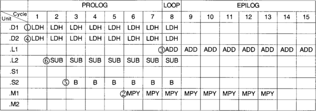
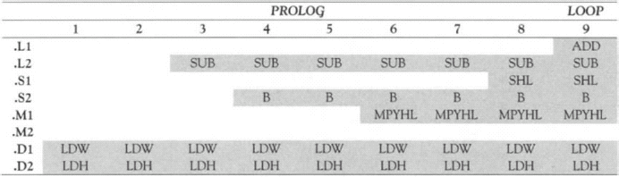
The next step for handwriting a pipelined code is to set up a scheduling table. To do so, the longest path must be identified in order to determine how long the table should be. Counting the latencies of each side, we see that the longest path is 8. This means that 7 prolog columns are required before entering the loop kernel. Thus, as shown in Table 7-1, the scheduling table consists of 15 columns (7 for prolog, 1 for loop kernel, 7 for epilog) and eight rows (one row for each functional unit). Epilog and prolog are of the same length.
The scheduling is started by placing the load instructions in parallel in cycle 1. These instructions are repeated at every cycle thereafter. The multiply instruction must appear five cycles after the loads (1 cycle for loads + 4 load delays), so it is scheduled into slot or cycle 6. The addition must appear two cycles after the multiply (1 cycle for multiply + 1 multiply delay), requiring it to be placed in slot or cycle 8, which is the loop kernel part of the code. The branch instruction is scheduled in slot or cycle 3 by reverse counting 5 cycles back from the loop kernel. The subtraction must occur before the branch, so it is scheduled in slot or cycle 2. The completed scheduling table appears in Table 7-2.
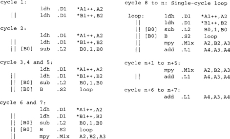
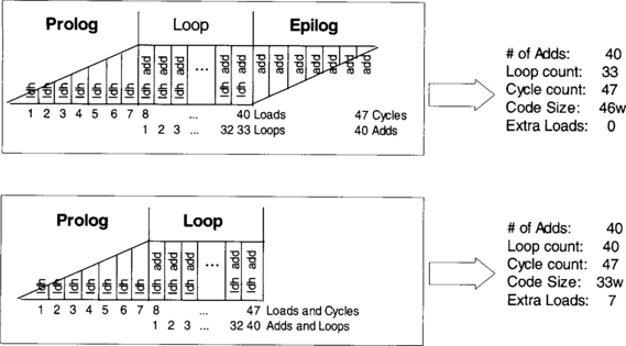
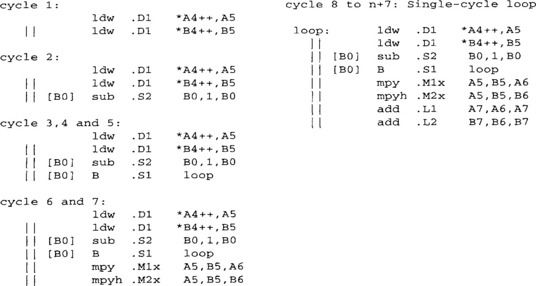
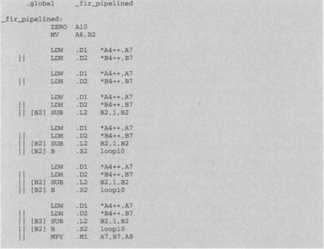
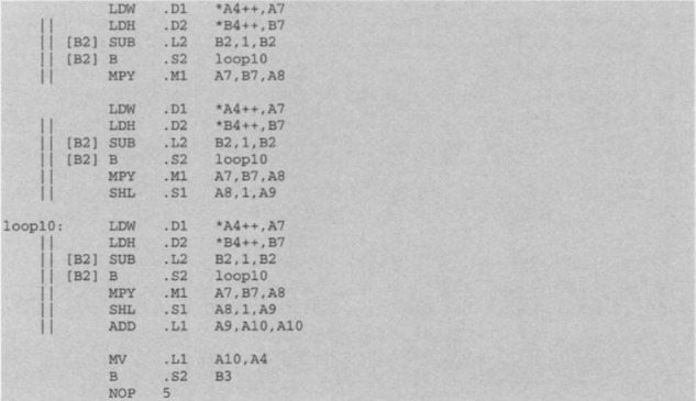
Next, the code is handwritten directly from the scheduling table as 7 prolog parallel instructions, 40 – 7=33 loop kernel parallel instructions, and 7 epilog parallel instructions. This hand-coded software pipelined code is shown in Figure 7-13. It can be seen that this pipelined code requires only 47 cycles to perform the dot-product 40 times. Note that, as shown in Figure 7-14, it is possible to eliminate the epilog instructions by performing the loop kernel instruction 40 instead of 33 times, leading to a lower code size and a higher number of loads.
Figures 7-15(b) and 7-15(c) show the dependency graph and the scheduling table, respectively, of the word-wide optimized dot-product code appearing in Figure 7-15(a). The corresponding hand-coded pipelined code is shown in Figure 7-16. This time, 28 cycles are required: 7 prolog instructions, 40/(2 word datatype) = 20 loop kernel instructions, and one extra add to sum the even and odd parts. Table 7-3 provides the number of cycles for different optimizations of the dot-product example discussed throughout the book. The interested reader is referred to the TI TMS320C6x Programmer’s Guide [2] for more details on how to handwrite software pipelined assembly code.
Table 7-3
| No optimization | 16 cycles * 40 iterations = | 640 |
| Parallel optimization | 15 cycles * 40 iterations = | 600 |
| Filling delay slots | 8 cycles * 40 iterations = | 320 |
| Word wide optimizations | 8 cycles * 20 iterations = | 160 |
| Software pipelined -LDH | 1 cycle * 40 loops + 7 prolog = | 47 |
| Software pipelined -LDW | 1 cycle * 20 loops + 7 prolog + 1 epilog = | 28 |
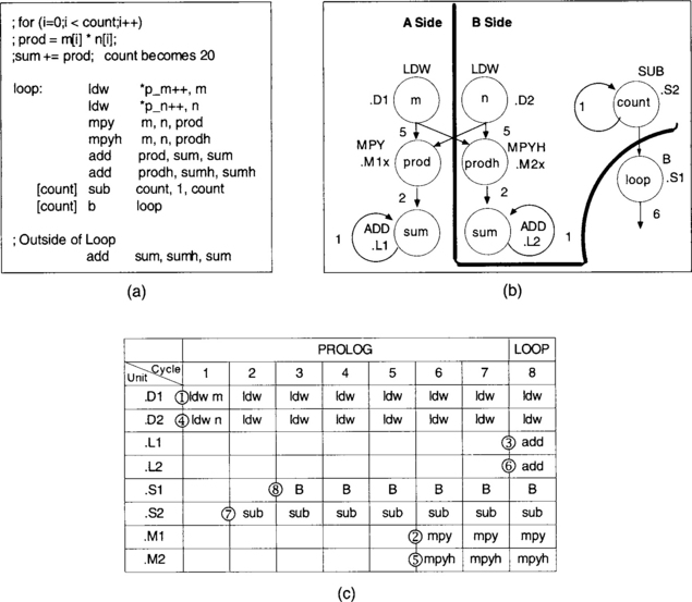
Figure 7-15 (a) Linear assembly dot-product code, (b) corresponding dependency graph, and (c) scheduling table.†
Multicycle loops – Let us now examine an example denoting a weighted vector sum c = a + r * b, where a and b indicate two arrays or vectors of size 40 and r a constant or scalar. Figure 7-17 shows the linear assembly code and the corresponding dependency graph to compute c. A problem observed in this dependency graph is that there are more than two loads/stores operations (i.e., the .D1 unit is assigned to two nodes). This, of course, is not possible in a single-cycle loop. Consequently, we must have two instead of one cycle loop. In other words, two parallel instructions are needed to compute the vector sum c per iteration.
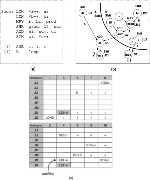
This time, the scheduling table consists of two sets of functional units arranged as shown in Figure 7-17. In this example, the length of the longest path is 10, which corresponds to the load-multiply-shift-add-store path. This means that there should be 10 cycle columns. However, this time the cycle number is set up by alternating between the two sets of functional units. The scheduling is started by entering the instructions for the longest path. The load LDH bi is placed in slot 1. MPY is placed in slot 6, five slots after slot 1 to accommodate for the load latencies. SHR is placed in slot 8, two slots after slot 6 to accommodate for the multiply latency. ADD is placed in slot 9, one slot after slot 8, and STH ci in the last slot 10. The other path is then scheduled. The loading LDH ai for this path must be done 5 slots or cycles before the ADD instruction. This would place LDH ai in slot 4. However, notice that the .D1 unit as part of the second loop cycle has already been used for STH ci and cannot be used at the same time. Hence, this creates a conflict which must be resolved. As indicated by the shaded boxes in Figure 7-17, the conflict is resolved either by using the .D2 unit in the second cycle loop or by using the .D1 unit in the first cycle loop.
7.4 C64x Improvements
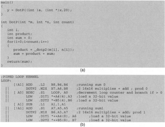
This section shows how the additional features of the C64x DSP can be used to further optimize the dot-product example. Figure 7-18(b) shows the C64x version of the dot-product loop kernel for multiplying two 16-bit values. The equivalent C code appears in Figure 7-18(a).
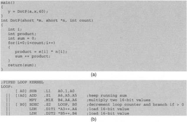
Now, by using the DOTP2 instruction of the C64x, we can perform two 16* 16 multiplications, reducing the number of cycles by one-half. This requires accessing two 32-bit values every cycle. As shown in Figure 7-19(a), in C, these can be achieved by using the intrinsic _dotp2 ( ) and by casting shorts as integers. The equivalent loop kernel code generated by the compiler is shown in Figure 7-19(b), which is a double-cycle loop containing four 16* 16 multiplications. The instruction LDW is used to bring in the required 32-bit values.
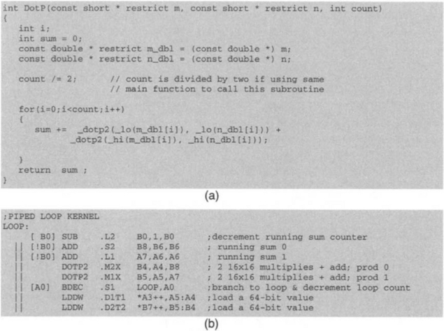
Considering that the C64x can bring in 64-bit data values by using the double-word loading instruction LDDW, the foregoing code can be further improved by performing four 16 * 16 multiplications via two DOTP2 instructions within a single-cycle loop, as shown in Figure 7-20(b). This way the number of operations is reduced by four-fold, since four 16* 16 multiplications are done per cycle. To do this in C, we need to cast short datatypes as doubles, and to specify which 32 bits of 64-bit data a DOTP2 is supposed to operate on. This is done by using the _1o ( ) and _hi ( ) intrinsics to specify the lower and the upper 32 bits of 64-bit data, respectively. Figure 7-20(a) shows the equivalent C code.
Lab. 4 Real-Time Filtering
The purpose of this lab is to design and implement a finite impulse response filter on the C6x. The design of the filter is done by using MATLAB™. Once the design is completed, the filtering code is inserted into the sampling shell program as an ISR to process live signals in real-time.
L4.1 Design of FIR Filter
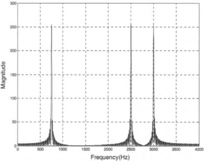
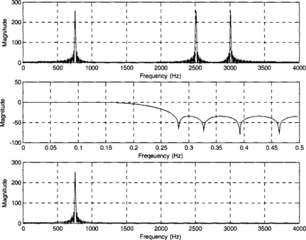
MATLAB or filter design packages can be used to obtain the coefficients for a desired FIR filter. To have a more realistic simulation, a composite signal may be created and filtered in MATLAB. A composite signal consisting of three sinusoids, as shown in Figure 7-21, can be created by the following MATLAB code:
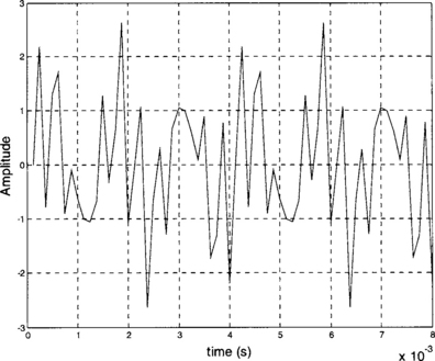
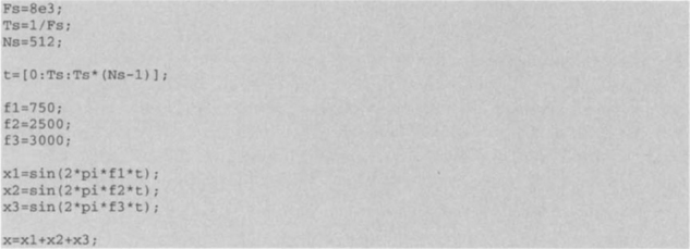
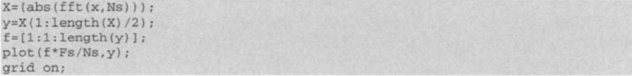
The signal frequency content can be plotted by using the MATLAB ‘fft’ function. Three spikes should be observed, at 750 Hz, 2500 Hz, and 3000 Hz. The frequency leakage observed on the plot is due to windowing caused by the finite observation period. A lowpass filter is designed here to filter out frequencies greater than 750 Hz and retain the lower components. The sampling frequency is chosen to be 8 kHz, which is common in voice processing. The following code is used to get the frequency plot shown in Figure 7-22:
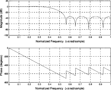
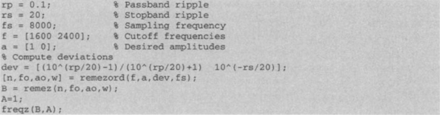
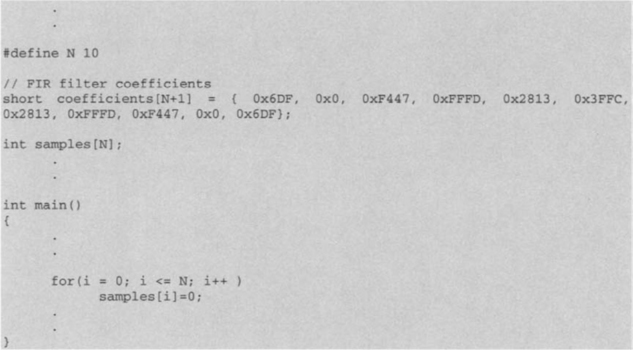
To design a FIR filter with passband frequency = 1600 Hz, stopband frequency = 2400 Hz, passband gain = 0.1 dB, stopband attenuation = 20 dB, sampling rate = 8000 Hz, the Parks-McClellan method is used via the ‘remez’ function of MATLAB [1]. The magnitude and phase response are shown in Figure 7-23, and the coefficients are given in Table 7-3. The MATLAB code is as follows:
Table 7-3
| Coefficient | Values | Q-15 Representation |
| B0 | 0.0537 | 0x06DF |
| B1 | 0.0000 | 0x0000 |
| B2 | −0.0916 | 0xF447 |
| B3 | −0.0001 | OxFFFD |
| B4 | 0.3131 | 0x2813 |
| B5 | 0.4999 | 0x3FFC |
| B6 | 0.3131 | 0x2813 |
| B7 | −0.0001 | 0xFFFD |
| B8 | −0.0916 | 0xF447 |
| B9 | 0.0000 | 0x0000 |
| B10 | 0.0537 | 0x06DF |
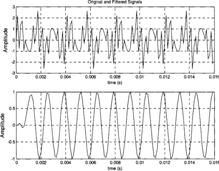
With these coefficients, the ‘filter’ function of MATLAB is used to verify that the FIR filter is actually able to filter out the 2.5 kHz and 3 kHz signals. The following MATLAB code allows one to visually inspect the filtering operation:
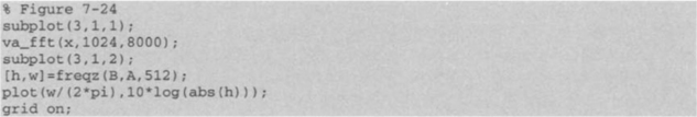
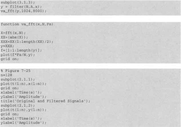
Looking at the plots appearing in Figures 7-24 and 7-25, we see that the filter is able to remove the desired frequency components of the composite signal. Observe that the time response has an initial setup time causing the first few data samples to be inaccurate. Now that the filter design is complete, let us consider the implementation of the filter.
L4.2 FIR Filter Implementation
An FIR filter can be implemented in C or assembly. The goal of the implementation is to have a minimum cycle time algorithm. This means that to do the filtering as fast as possible in order to achieve the highest sampling frequency (the smallest sampling time interval). Initially, the filter is implemented in C, since this demands the least coding effort. Once a working algorithm in C is obtained, the compiler optimization levels (i.e., –o2, –o3) are activated to reduce the number of cycles. An implementation of the filter is then done in hand-coded assembly, which can be software pipelined for optimum performance. A final implementation of the filter is performed in linear assembly, and the timing results are compared.
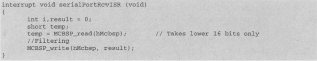
The difference equation ![]() is implemented to realize the filter. Since the filter is implemented on the DSK, the coding is done by modifying the sampling program in Lab 2, which uses an ISR that is able to receive a sample from the serial port and send it back out without any modification.
is implemented to realize the filter. Since the filter is implemented on the DSK, the coding is done by modifying the sampling program in Lab 2, which uses an ISR that is able to receive a sample from the serial port and send it back out without any modification.
When using the C6711 DSK together with the audio daughter card, the received data from McBSP1 is 32-bit wide with the most significant 16 bits coming from the right channel, and the least significant 16 bits coming from the left channel. The FIR filter implementation on the EVM is discussed in Section L4.4.
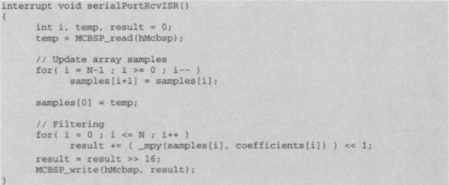
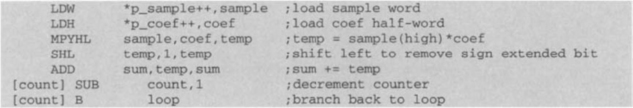
Considering Q-15 representation here, the mpy instruction is utilized to multiply the lower part of a 32-bit sample (left channel) by a 16-bit coefficient. In order to store the product in 32 bits, it has to be left shifted by one to get rid of the extended sign bit. Now, to export the product to the codec output, it must be right shifted by 16 to place it in the lower 16 bits. Alternatively, the product may be right shifted by 15 without removing the sign bit.
To implement the algorithm in C, the _mpy ( ) intrinsic and the shift operators ‘<<’ and ‘>>’ should be used as follows:
![]()
![]()
Here, result and sample are 32 bits wide, while coefficient is 16 bits wide. The intrinsic _mpy ( ) multiplies the lower 16 bits of the first argument by the lower 16 bits of the second argument. Therefore, the lower 16 bits of sample is used in the multiplication.
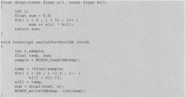
For the proper operation of the FIR filter, it is required that the current sample and N-1 previous samples be processed at the same time, where N is the number of coefficients. Hence, the N most current samples have to be stored and updated with each incoming sample. This can be done easily via the following code:
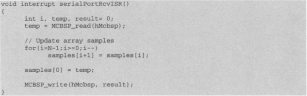
Here, as a new sample comes in, each of the previous samples is moved into the next location in the array. As a result, the oldest sample sample [N], is discarded, and the newest sample, temp, is put into sample [0].
This approach adds some overhead to the ISR, but for now it is acceptable, since at a sampling frequency of 8 kHz, there is a total of 18,750 cycles are available, [1/(8 kHz /150 MHz) = 18,750], between consecutive samples, considering that the DSK runs at 150 MHz. The total overhead for this manipulation is 358 cycles without any optimization. It should be noted that the proper way of doing this type of filtering is by using circular buffering. The circular buffering approach will be discussed in Lab 5.
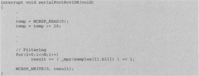
Now that the N most current samples are in the array, the filtering operation may get started. All that needs to be done, according to the difference equation, is to multiply each sample by the corresponding coefficient and sum the products. This is achieved by the following code:
To complete the FIR filter implementation, we need to incorporate the filter coefficients previously designed into the C program. This is accomplished by modifying the sampling program in Lab 2 as follows:
The filtering program can now be built and run. Using a function generator and an oscilloscope, it is possible to verify that the filter is working as expected. The output of the function generator should be connected to the line-in jack of the audio daughter card, and the line-out jack of the daughter card to the input of the oscilloscope. As the input frequency is increased, it is seen that the signal attenuation starts at 1.6 kHz and dies out at 2.4 kHz. Note that the nearest sampling frequency should be selected, since the sampling frequencies of the audio daughter card are limited. As a result, the frequencies for passband and stopband are considered to be 1.46 kHz and 2.20 kHz with the sampling frequency of 7324.22 Hz.
Given that a working design is reached, it is time to start the optimization of the filtering algorithm. The first step in optimization is to use the compiler optimizer. The optimizer can be invoked by choosing Project → Options from the CCS menu bar. This option will invoke a dialog box, as shown in Figure 7-26. In this dialog box, select Basic in the Category field, and then choose the desired optimization level from the pull-down list in the Opt Level field. Table 7-4 summarizes the timing results for different optimization levels.
Table 7-4
Timing cycles for different builds.
| Build Type | Number of Cycles |
| Compile without optimization | 670 |
| Compile with −o0 | 396 |
| Compile with −o1 | 327 |
| Compile with −o2/–o3 | 159 |
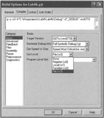
As can be seen from Table 7-4, the number of cycles diminishes as the optimization level is increased. It is important to remember that because the compiler optimizer changes the flow of a program, the debugger may not work in some cases. Therefore, it is advised that one make sure a program works correctly before performing any compiler optimization.
Before doing the linear assembly implementation, the code is written in assembly to see how basic optimization methods such as placing instructions in parallel, filling delay slots, loop unrolling, and word-wide optimization affect the timing cycle of the code.
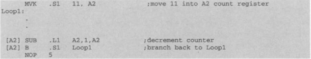
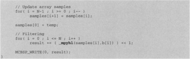
To perform the operation of multiplying and adding N coefficients, a loop needs be set up. This can be done by using a branch instruction. A counter is required to exit the loop once N iterations have been performed. For this purpose, one of the conditional registers (A1, A2, B0, B1 or B2) is used. No other register allows for conditional testing. Adding [A2] in front of an instruction permits the processor to execute the instruction if the value in A2 does not equal zero. If A2 contains zero, the instruction is skipped, noting that an instruction cycle is still consumed. The .S1 unit may be used to perform the move constant and branch operations. The value in the conditional register A2 decreases by using a subtract instruction. Since the subtract operation should stop if the value drops below zero, this conditional register is mentioned in the SUB instruction to execute it only if the value is not equal to zero. The programmer should remember to add five delay slots for the branch instruction. The code for this loop is as follows:
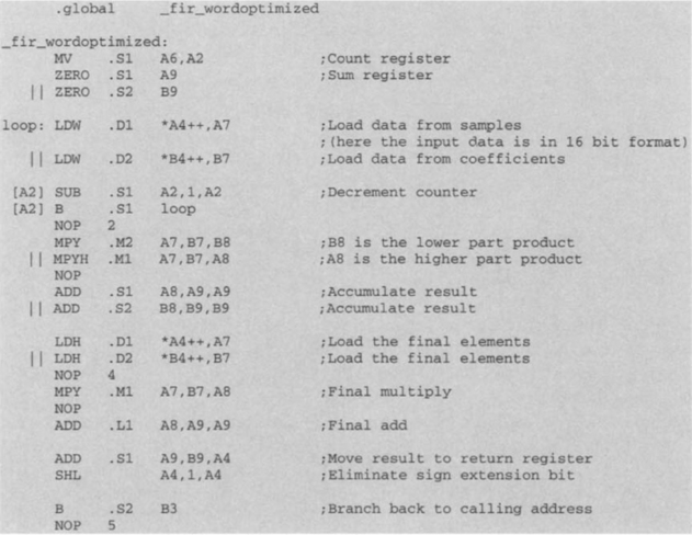
We can now start adding instructions to perform the multiplication and accumulation of the values. First, those values that are to be multiplied need to be loaded from their memory locations into the CPU registers. This is done by using load word (LDW) and load half-word (LDH) instructions. Upon executing the load instructions, the pointer is post-incremented so that it is pointed to the next memory location. Once the values have appeared in the registers (four cycles after the load instruction), the MPY instruction is used to multiply them and store the product in another register. Then, the summation is performed by using the ADD instruction. The completed assembly program is as follows:
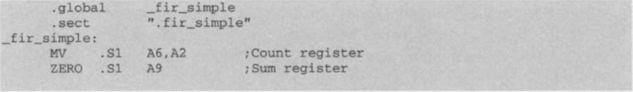
The preceding code is a C callable assembly function. To call this function from C, a function declaration must be added as external (extern) without any arguments. The arguments to the function are passed via registers A4, B4 and A6. The return value is stored in A4. Here, the pointers to the arrays are passed in A4 and B4 as the first two arguments and the number of iterations in A6 as the third argument. The return address from the function is stored in B3. Therefore, a final branch to B3 is required to return from the function. For a complete explanation of calling assembly functions from C, see the TI TMS320C6x Optimizing C Compiler User’s Guide [2].
The directive .sect is used to place the code in the appropriate memory location. Running the code from the external SDRAM memory takes a total of 1578 cycles for the assembly function to complete. To move the code into the internal memory so that it runs faster, the linker command file should be modified by replacing .fir_simple ≥ CEO with .fir_simple ≥ IRAM. Running the code from the internal memory results in 313 cycles. Notice that only the assembly function is running in the internal program memory; the rest of the ISR is located in the external memory and still runs slow, taking a total of 2938 cycles. It is possible to move the entire ISR into the internal memory to obtain a faster execution. The CODE_SECTION pragma can be used for this purpose. By adding the following line to the code, the entire ISR is placed in the internal memory, leading to a total of 754 cycles:
![]()
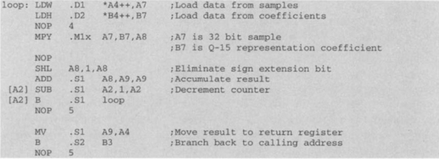
To optimize the foregoing function, basic optimization methods, such as placing instructions in parallel, filling delay slots, and loop unrolling, are applied. Examining the code, one sees that some of the instructions can be placed in parallel. Because of operand dependencies, care must be taken not to schedule parallel instructions that use previous operands as their operands. The two initial load instructions are independent and can be made to run in parallel. Looking at the rest of the program, we can see that the operands are dependent on the previous operands; hence, no other instructions are placed in parallel.
To reduce the cycles taken by the NOP instructions, we can use the delay slot filling technique. For example, as the load instructions are executed in parallel, it is possible to schedule the subtraction of the loop counter in place of their NOPs. The branch instruction takes five cycles to execute. It is therefore possible to slide the branch instruction four slots up to get rid of its NOPs. Incorporating these optimizations, we can rewrite the function as follows:
By filling delay slots, the number of cycles is reduced. In repetitive loops such as this one, it is seen that the branch instruction takes up extra cycles that can be eliminated. As just mentioned, one method to do this elimination is to fill the delay slots by sliding the branch instruction higher in the execution phase, thus filling the latencies associated with branching. Another method for reducing the latencies is to unroll the loop. However, notice that loop unrolling eliminates only the last latency of the branch. Since, in the preceding delay filled version, the branch latency has no effect on the number of cycles, loop unrolling does not achieve any further improvement in timing.
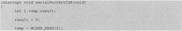
To perform word-wide optimization, the ISR has to be modified to store a sample into 16 bits rather than 32 bits. This can be simply achieved by using a variable of type short. The following code stores a sample into a short variable, temp, assuming that the result is 32 bits.
Using word-wide optimization, one needs to load two consecutive 16 bit values in memory with a single load-word instruction. This way, the input register contains two values, one in the lower and the other in the upper part. The instructions MPYH and MPY can be used to multiply the upper and lower parts, respectively. The following assembly code shows how this is done for the FIR filtering program:
Notice that since two loads are done consecutively, it takes half the amount of time to loop through the program. When calling this function, the value passed in A6 must be the truncated N/2, where N is the number of coefficients of the FIR filter. In our case, we have 11 coefficients requiring five iterations plus an additional multiply and accumulate. With this code, it is possible to bring down the number of cycles to 101. The timing cycles for the aforementioned optimizations are listed in Table 7-5.
Table 7-5
Timing cycles for different optimizations.
| Optimization | Number of Cycles |
| Un-optimized assembly | 313 |
| Delay slot filled assembly | 141 |
| Word optimized assembly | 101 |
L4.2.1 Handwritten Software-pipelined Assembly
To produce a software-pipelined version of the code, it is required to first write it in symbolic form without any latency or register assignment. The following code shows how to write the FIR program in a symbolic form:
To handwrite software-pipelined code, a dependency graph of the loop must be drawn and a scheduling table be created from it. The software-pipelined code is then derived from the scheduling table. To draw a dependency graph, we start by drawing nodes for the instructions and symbolic variable names. Then we draw lines or paths that show the flow of data between nodes. The paths are marked by the latencies of the instructions of their parent nodes.
After the basic dependency graph is drawn, functional units have to be assigned. Then, a line is drawn between the two sides of the CPU so that the workload is split as equally as possible. In the preceding FIR program, the loads should be done one on each side, so that they run in parallel. It is up to the programmer on which side to place the rest of the instructions to divide the workload equally between the A-side and B-side functional units. The completed dependency graph for the FIR program is shown in Figure 7-27.
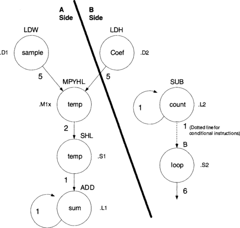
The next step for handwriting a pipelined code is to set up a scheduling table. To do so, the longest path must be identified to determine how long the table should be. Counting the latencies of each side, one sees that the longest path located on the left side is 9. Thus, eight prolog columns are required in the table before entering the main loop. There need to be eight rows (one for each functional unit) and nine columns in the table. The scheduling is started by placing the parallel load instructions in slot 1. The instructions are repeated at every loop thereafter. The multiply instruction must appear five slots after the loads, so it is scheduled into slot 6. The shift must appear two slots after the multiply, and the add must appear after the shift instruction, placing it in slot 9, which is the loop kernel part of the code. The branch instruction is scheduled in slot 4 by reverse counting five cycles back from the loop kernel. The subtraction must occur before the branch, so it is scheduled in slot 3. The completed scheduling table appears in Table 7-6.
The software-pipelined code is handwritten directly from the scheduling table as eight parallel instructions before entering a loop that completes all the adds. The resulting code, with which the number of cycles is reduced to 72, is as follows:
L4.2.2 Assembly Optimizer Software-Pipelined Assembly
Since handwritten pipelined codes are time-consuming to write, linear assembly is usually used to generate pipelined codes. In linear assembly, latencies, functional units and register allocations do not need to be specified. Instead, symbolic variable names are used to write a sequential code with no delay slots (NOPs). The file extension for a linear assembly file is .sa. The assembly optimizer is automatically invoked if a file in a CCS project has a .sa extension. The assembly optimizer turns a linear assembly code into a pipelined code. Notice that the optimization level option in C also affects the optimization of linear assembly.
A code line in linear assembly consists of five fields: label, mnemonic, unit specifier, operand list, and comment. The general syntax of a linear assembly code line is:
![]()
Fields in square brackets are optional. A label must begin in column 1 and can include a colon. A mnemonic is an instruction such as MPY or an assembly optimizer directive such as .proc. Notice that a mnemonic will be interpreted as a label if it begins in column 1. At least one blank space should be placed in front of a mnemonic when there is no label. A mnemonic becomes a conditional instruction when it is preceded by a register or a symbolic variable within two square brackets. A unit specifier specifies the functional unit performing the mnemonic. Operands can be symbols, constants, or expressions and should be separated by commas. Comments begin with a semicolon. Comments beginning in column 1 can begin with either an asterisk or a semicolon.
In writing code in linear assembly, the assembly optimizer must be supplied with the right kind of optimization information. The first such piece of information is which parts should be optimized. The optimizer considers only code between the directives .proc and .endproc. Symbolic variable names are used to allow the optimizer to select which registers to use. This is done by using the .reg directive together with the names of the variables. Also, registers that contain input arguments, such as variables passed to a function, must be specified. The registers declared to contain input arguments cannot be modified and have to be declared as operands of the .proc statement. To connect the input register arguments to the symbolic variable names, the move instruction, mv, is used. Registers that contain output values upon exiting the procedure must be declared as arguments to the .endproc directive.
To write the FIR code in linear assembly, we start by creating the main loop and then add the load, multiply, and add instructions. Since two pointers to two arrays and an integer are passed to the function, we must declare registers A4, B4 and A6 as part of the .proc directive. Also, register A4 is used for returning values, so it needs to appear as part of the .endproc directive. The preserved register B3 is indicated as an argument in both of these directives. To connect the symbolic variable names to the input registers, the mv instruction is used. And finally, the optimizer is told that the loop is to be performed a minimum of 11 times by inserting the .trip directive. The final code is as follows:
Using this code, we obtain a timing outcome of 72 cycles, which is the same as the timing obtained by the handwritten software-pipelined assembly.
To summarize the programming approach, start writing your code in C, and then use the optimizer to achieve a faster code. If the code is not as fast as expected, you may write it in assembly and incorporate the aforementioned simple optimization techniques. However, it is usually easier and more efficient to rewrite your code in linear assembly, since the assembly optimizer attempts to create pipelined code for you. Figure 7-28 illustrates the code development flow to get an optimum performance on the C6x. If, at the end, none of these approaches provide a satisfactory timing cycle, you are left no choice but to rewrite your code in hand-coded pipelined assembly. Appendix A (Quick Reference Guide) includes an optimization checklist for writing DSP application programs.

L4.3 Floating-Point Implementation
Implementing the FIR filter on the floating-point C67x takes relatively less effort. Since the hardware is capable of multiplying and adding floating point numbers, Q-format number manipulation is not required. However, in general, the floatingpoint code is slower, because floating-point operations have more latencies than their fixed-point counterparts. As is shown shortly, the FIR filter interrupt and function are modified for the floating-point execution. The code written in C is fairly simple. The coefficients are entered directly as float. The data buffer is declared as float, and a sample is initially read as an integer and then typecast to a float. Reversely, the outcome is typecasted into integer.
You can view your C source code interleaved with disassembled code in CCS. To view this mixed mode, after loading the program into the DSP, open the source file by double-clicking on it from the Project View panel. Select View → Mixed Source/ASM from the menu. Using this mixed mode, it can be verified that the compiler is actually using the MPYSP and ADDSP instructions to perform the floating-point multiply and add rather than calling a separate function to do them in software. The code is as follows:
All the programs associated with this lab can be loaded from the accompanying CD.
L4.4 EVM Implementation
Since, on EVM, data are acquired from the codec through McBSP0, different than that of DSK, appropriate changes need to be made. As discussed in the preceding section, data samples from the left channel are stored in the higher 16-bit of integer variable. In order to maintain compatibility with the DSK code, the intrinsic_MPYHL is used instead of _MPY for the multiplication of 32-bit samples with 16-bit coefficients.
Alternatively, the sample in the DRR can be right shifted by 16 and stored in the lower 16-bit, followed by the MPY instruction, as shown in the code that follows:
The output value stored in result contains Q-31 format data with the extra bit at the least significant bit. Data in the higher 16-bit are considered as Q-15 format and exported to the left channel, thus no alignment of data is necessary.