Software Tools
Programming most DSP processors can be done either in C or assembly. Although writing programs in C would require less effort, the efficiency achieved is normally less than that of programs written in assembly. Efficiency means having as few instructions or as few instruction cycles as possible by making maximum use of the resources on the chip.
In practice, one starts with C coding to analyze the behavior and functionality of an algorithm. Then, if the required processing rate is not met by using the C compiler optimizer, the time-consuming portions of the C code are identified and converted into assembly, or the entire code is rewritten in assembly. In addition to C and assembly, the C6x allows writing code in linear assembly. Figure 4-1 illustrates the code efficiency versus coding effort for three types of source files on the C6x: C, linear assembly, and hand-optimized assembly. As can be seen, linear assembly provides a good compromise between code efficiency and coding effort.
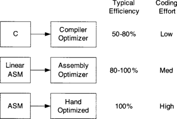
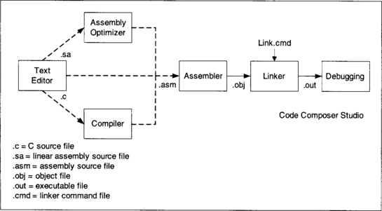
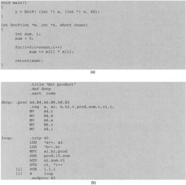
Figure 4-2 shows the steps involved for going from a source file (.c extension for C, .asm for assembly, and .sa for linear assembly) to an executable file (.out extension). Figure 4-3 lists the .c and .sa versions of the dot-product example to see what they look like. The assembler is used to convert an assembly file into an object file (.obj extension). The assembly optimizer and the compiler are used to convert, respectively, a linear assembly file and a C file into an object file. The linker is used to combine object files, as instructed by the linker command file (.cmd extension), into an executable file. All the assembling, linking, compiling, and debugging steps have been incorporated into an integrated development environment (IDE) called Code Composer Studio (CCS or CCStudio). CCS provides an easy-to-use graphical user environment for building and debugging C and assembly codes on various target DSPs.
4.1 C6x DSK/EVM Target Boards
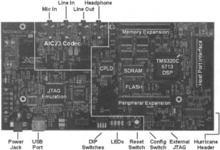
Upon the availability of either a DSK or an EVM board, an executable file can be run on an actual C6x processor. In the absence of such boards, CCS can be configured to simulate the execution process. As shown in Figure 4-4, the C6713 DSK board is a DSP system which includes a C6713 DSP chip operating at 225 MHz with 4/4/256 Kbytes memory for L1D data cache/L1P program cache/L2 memory, respectively, 8 Mbytes of onboard SDRAM (synchronous dynamic RAM), 512 Kbytes of flash memory, and a 16-bit stereo codec AIC23 with sampling frequency of 8 kHz to 96 kHz. The C6416 DSK board includes a C6416 DSP chip operating at 600 MHz with 16/16/1024 Kbytes memory for L1D data cache/L1P program cache/L2 cache, respectively, 16 Mbytes of onboard SDRAM, 512 Kbytes of flash memory, and AIC23 codec. The C6711 DSK board includes a C6711 DSP chip operating at 150 MHz with 4/4/64 Kbytes of memory for L1D data cache/L1P program cache/L2 cache, 16 Mbytes of onboard SDRAM, 128 Kbytes flash memory, a 16-bit codec AD535 having a fixed sampling frequency of 8 kHz, and a daughter card interface to which a PCM3003 audio daughter card can be connected for changing sampling frequency.
As shown in Figure 4-5(a), the C6701/C6201 EVM board is a DSP system which includes a C6701 (or C6201) chip, external memory, A/D capabilities, and PC host interfacing components. The functional diagram of the EVM board appears in Figure 4-5(b). The board has a 16-bit codec CS4231A whose sampling frequency can be changed from 5.5 kHz to 48 kHz.
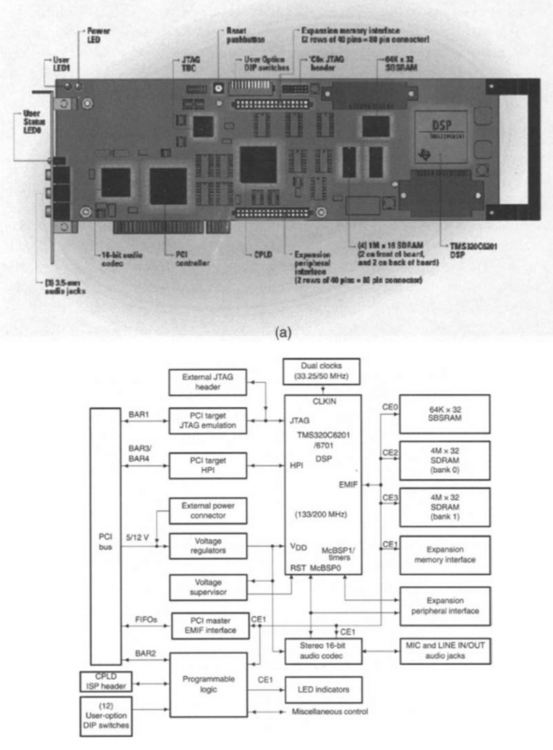
The memory residing on the EVM board consists of 32 Mbytes SDRAM running at 100 MHz and 256 Kbytes SBSRAM (synchronous burst static RAM) running at 133 MHz, a faster, but more expensive, memory as compared to SDRAM. A voltage regulator on the board is used to provide 1.8V or 2.5V for the C6x core and 3.3V for its memory and peripherals, and 5V for audio components.
4.2 Assembly File
Similar to other assembly languages, the C6x assembly consists of four fields: label, instruction, operands, and comment. (See Figure 3-4.) The first field is the label field. Labels must start in the first column and must begin with a letter. A label, if present, indicates an assigned name to a specific memory location that contains an instruction or data. Either a mnemonic or a directive constitutes the instruction field. It is optional for the instruction field to include the functional unit which performs that particular instruction. However, to make codes more understandable, the assignment of functional units is recommended. If a functional unit is specified, the data path must be indexed by 1 for the A side and 2 for the B side. A parallel instruction is indicated by a double pipe symbol (||), and a conditional instruction by a register appearing in brackets in the instruction field. As the name operand implies, the operand field contains arguments of an instruction. Instructions require two or three operands. Except for store instructions, the destination operand must be a register. One of the source operands must be a register, the other a register or a constant. After the operand field, there is an optional comment field that, if stated, should begin with a semicolon (;).
4.2.1 Directives
Directives are used to indicate assembly code sections and to declare data structures. It should be noted that assembly statements appearing as directives do not produce any executable code. They merely control the assembling process by the assembler. Some of the widely used assembler directives are:
.sect “name” directive, which defines a section of code or data named “name”.
.int, .long, or .word directive, which reserves 32 bits of memory initialized to a value.
.short or .half directive, which reserves 16 bits of memory initialized to a value.
.byte directive, which reserves 8 bits of memory initialized to a value.
Note that in the TI common object file format (COFF), the directives .text, .data, .bss are used to indicate code, initialized constant data, and uninitialized variables, respectively. Other directives often used include .set directive, for assigning a value to a symbol, .global or .def directive, to declare a symbol or module as global so that it may be recognized externally by other modules, and .end directive, to signal the termination of assembly code. The directive .global acts as a .def directive for defined symbols and as a .ref directive for undefined symbols.
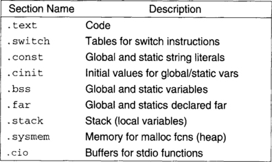
At this point, it should be mentioned that the C compiler creates various sections indicated by the directives .text, .switch, .const, .cinit, .bss, .far, .stack, .sysmem, .cio. Figure 4-6 lists some common compiler sections. For a complete listing of directives, refer to the TI TMS320C6x Assembly Language Tools User’s Guide [1].
4.3 Memory Management
The external memory used by a DSP processor can be either static or dynamic. Static memory (SRAM) is faster than dynamic memory (DRAM), but it is more expensive, since it takes more space on silicon. DRAMs also need to be refreshed periodically. A good compromise between cost and performance is achieved by using SDRAM (Synchronous DRAM). Synchronous memory requires clocking, as compared to asynchronous memory, which does not.
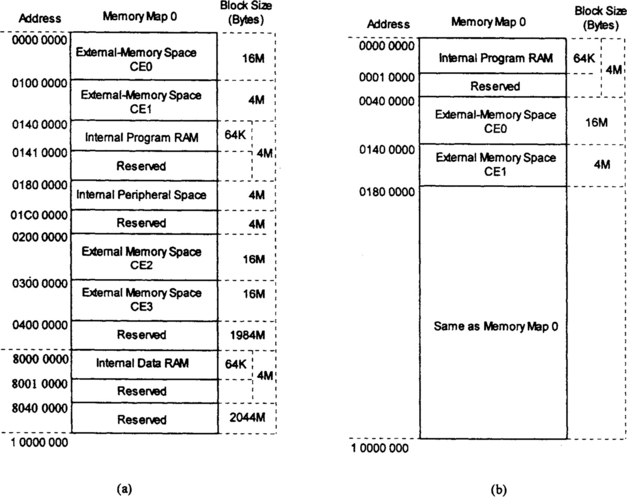
Given that the address bus is 32 bits wide, the total memory space consists of 232 = 4 Gbytes. On the EVM, this space is divided, according to a memory map, into the internal program memory (PMEM), internal data memory (DMEM), internal peripherals, and external memory spaces named CE0, CE1, CE2, and CE3. There are two memory map configurations: memory map 0 and memory map 1. Figures 4-7 (a) and 4-7(b) illustrate these two memory maps. On the DSK, there is no separation between internal program and data memory. For the lab exercises in this book, the EVM board is configured based on its memory map 1 as shown in Figure 4-7(c), and the DSK board based on its memory map 1 as shown in Figure 4-7 (d).

The external memory ranges CE0, CE1, CE2, and CE3 support synchronous (SBSPvAM, SDRAM) or asynchronous (SRAM, ROM, and so forth) memory, accessible as bytes (8 bits), halfwords (16 bits), or words (32 bits). The on-chip peripherals and control registers are mapped into the memory space. A listing of the memory-mapped registers is provided in Appendix A (Quick Reference Guide).
The internal data memory is organized into memory banks so that two loads or stores can be done simultaneously. As long as data are accessed from different banks, no conflict occurs. However, if data are accessed from the same bank in one instruction, a memory conflict occurs and the CPU is stalled by one cycle.
If a program fits into the on-chip or internal memory, it should be run from there to avoid delays associated with accessing off-chip or external memory. If a program is too big to be fitted into the internal memory, most of its time-consuming portions should be placed into the internal memory for efficient execution. For repetitive codes, it is recommended that the internal memory is configured as cache memory. This allows accessing external memory as seldom as possible and hence avoiding delays associated with such accesses.
4.3.1 Linking
Linking places code, constant, and variable sections into appropriate locations in memory as specified in the .cmd linker command file. Also, it combines several .obj object files into the final executable .out output file. A typical command file corresponding to the DSK memory map 1 is shown below in Figure 4-8.
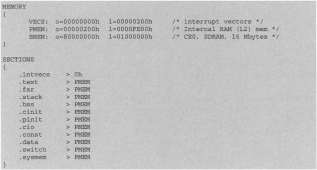
The first part, MEMORY, provides a description of the type of physical memory, its origin and its length. The second part, SECTIONS, specifies the assignment of various code sections to the available physical memory.
4.4 Compiler Utility
The build feature of CCS can be used to perform the entire process of compiling, assembling, and linking in one step via the activation of the utility c16x and stating the right options for it. The following command shows how this utility is used within CCS for building the source files file1.c, file2.asm, and file3.sa:
![]()
The option –g adds debugger specific information to the object file for debugging purposes. The option –s provides an interlisting of C and assembly. For file1.c, the C compiler, for file2.asm the assembler, and for file3.sa, the assembly optimizer (linear assembler) are invoked. The option –z invokes the linker, placing the executable code in file.out if the –o option is used. Otherwise, the default file a.out is created. The option –m provides a map file (file.map), which includes a listing of all the addresses of sections, symbols and labels. The option −1 specifies the run-time support library rts6700.lib for linking files on the C6713 processor. Table 4-1 lists some frequently used options. Refer to the TI Optimizing C Compiler manual [2] for a complete list of available options.
Table 4-1
| Options | Description | Tool |
| −mv6700 | Generate ’C67x code (’C62x is default) | Comp/Asm |
| −g | Enables src-level symbolic debugging | Comp/Asm |
| −mg | Enables minimum debug to allow profiling | Compiler |
| −s | Interlist C statements into assembly listing | Compiler |
| −o | Invoke optimizer (-o0, -o1, -o2/ -o, -o3) | Compiler |
| −pm | Combine all C source files before compile | Compiler |
| −mt | No aliasing used | Compiler |
| −ms | Minimize code size (-ms0/ -ms, -ms1, -ms2) | Compiler |
| −z | Invokes linker | Linker |
| −o | Output file name | Linker |
| −m | Map file name | Linker |
| −c | Auto -Init C variables (-cs turns off autoinit) | Linker |
| −1 | Link -in libraries (small -L) | Linker |
The compiler allows four levels of optimizations to be invoked by using –oO, –o1, –o2, –o3. Debugging and full-scale optimization cannot be done together, since they are in conflict; that is, in debugging, information is added to enhance the debugging process, while in optimizing, information is minimized or removed to enhance code efficiency. In essence, the optimizer changes the flow of C code, making program debugging very difficult.
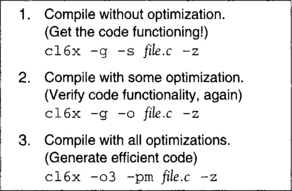
As shown in Figure 4-9, a good programming approach would be first to verify that the code is properly functioning by using the compiler with no optimization (-gs option). Then, use full optimization to generate an efficient code (-o3 option). It is recommended that an intermediary step be taken in which some optimization is done without interfering with source level debugging (-go option). This intermediary step can reverify code functionality before performing full optimization. It should be pointed out that full optimization may change memory locations outside the scope of the C code. Such memory locations must be declared as ‘volatile’ to prevent compiling errors.
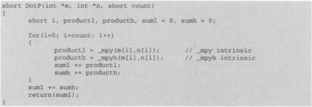
As a step to further optimize C codes, it is recommended that intrinsics be used wherever possible. Intrinsics are functions similar to math functions as part of the runtime support library. Intrinsics allow the C compiler to directly access the hardware while preserving the C environment. As an example, instead of using the multiply operator * in C, the intrinsic _mpy ( ) can be used to tell the compiler to use the C6x instruction MPY. Figure 4-10 shows the intrinsic version of the dot-product C code. A list of the C6x intrinsics is provided in Appendix A (Quick Reference Quide).
4.5 Code Initialization
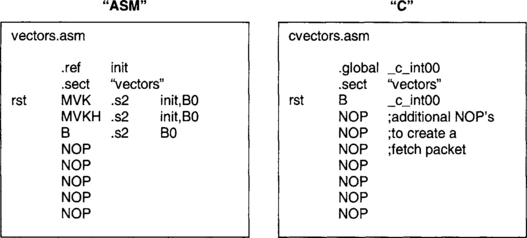
All programs start by going through a reset initialization code. Figure 4-11 illustrates both the C and assembly version of a typical reset initialization code. This initialization is for the purpose of starting at a previously defined initial location. Upon power up, the system always goes to the reset location in memory, which normally includes a branch instruction to the beginning of the code to be executed. The reset code shown in Figure 4-11 takes the program counter to a globally defined location in memory named init or _c_int00.
As indicated in Figure 4-12, when writing in assembly, an initialization code is needed to create initialized data and variables, and to copy initialized data into corresponding variables. Initialized values are specified by using .byte, .short, or .int directives. Uninitialized variables are specified by using .usect directive. The first, second, and third arguments of this directive denote section name, size in bytes, and data alignment in bytes, respectively. Before calling the main function or subroutine, another initialization code portion is usually needed to set up registers and pointers, and to move data to appropriate places in memory.
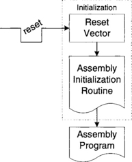
Figure 4-13 provides the initialization code for the dot-product example in which initialized data values appear for three initialized data arrays labeled Tabel_a, Tabel_x, and Tabel_y. In addition, three variable sections called a, x, and y aredeclared. The second part of the initialization code copies the initialized data intothe corresponding variables. The setup code for calling the dot-product routine isalso shown in this figure.
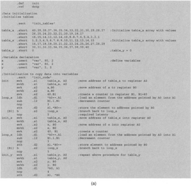
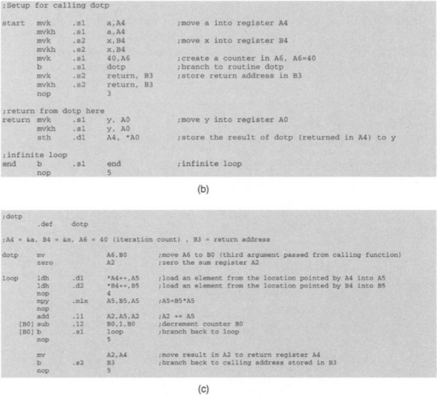
Figure 4-13 (a) Initialization code for dot-product example, (b) setup code for calling dot product routine, and (c) dot product routine.†
As far as C coding is concerned, the C compiler uses boot.c in the run-time support library to perform the initialization before calling main ( ). The –c option activates boot.c to autoinitialize variables. This is illustrated in Figure 4-14.
4.5.1 Data Alignment
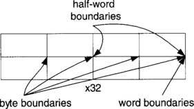
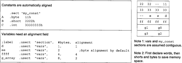
The C6x allows byte, half-word, or word addressing. Consider a word-format representation of memory as shown in Figure 4-15. There are four byte boundaries, two half-word (or short) boundaries, and one word boundary per word. The C6x always accesses data on these boundaries depending on the datatype specified; that is, it always accesses aligned data. When specifying an uninitialized variable section .usect, it is required to specify the alignment as well as the total number of bytes. The examples appearing in Figure 4-16 show data alignment for both constants and variables.
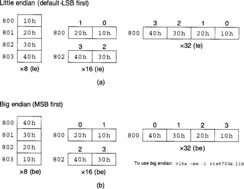
Data in memory can be arranged either in little- or big-endian format. Little-endian (le) means that the least significant byte is stored first. Figure 4-17 (a) shows storing .int 40302010h in little-endian format for byte, half-word, and word access addressing. In big-endian (be) format, shown in Figure 4-17(b), the most significant byte is stored first. Little-endian is the format normally used in most applications. Additional data alignment examples are shown in Figure 4-17(c), based on the little-endian data format appearing in Figure 4-17(a).
Lab 1 Getting Familiar with Code Composer Studio
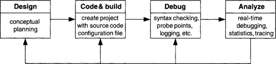
Code Composer Studio™ (CCStudio or CCS) is a useful integrated development environment (IDE) that provides an easy-to-use software tool to build and debug programs. In addition, it allows real-time analysis of application programs. Figure 4-18 shows the phases associated with the CCS code development process. During its set-up, CCS can be configured for different target DSP boards (for example, C6711 DSK, C6416 DSK, C6701 EVM, C6xxx Simulator). The version used throughout the book is based on CCS 2.2, the latest version at the time of this writing.
CCS provides a file management environment for building application programs. It includes an integrated editor for editing C and assembly files. For debugging purposes, it provides breakpoints, data monitoring and graphing capabilities, profiler for benchmarking, and probe points to stream data to and from the target DSP. This tutorial lab introduces the basic features of CCS that are needed in order to build and debug an application program. To become familiar with all of its features, one should go through the TI CCS Tutorial and TI CCS User’s Guide manuals [1–2]. The real-time analysis and scheduling features of CCS will be covered later, in Labs 7 and 8.
This lab demonstrates how a simple multifile algorithm can be compiled, assembled and linked by using CCS. First, several data values are consecutively written to memory. Then, a pointer is assigned to the beginning of the data so that they can be treated as an array. Finally, simple functions are added in both C and assembly to illustrate how function calling works. This method of placing data in memory is simple to use and can be used in applications in which constants need to be in memory, such as filter coefficients and FFT twiddle factors. Issues related to debugging and benchmarking are also covered in this lab.
The lab programs can be downloaded from the accompanying CD-ROM for different DSP target boards. Six versions of the lab programs appear on the CD. These versions correspond to (a) C6713 DSK, (b) C6416 DSK, (c) C6711 DSK together with a daughter card, (d) C6711 DSK without a daughter card, (e) C6701/C6201 EVM, and (f) simulator.
L1.1 Creating Projects
Let us consider all the files required to create an executable file; that is, .c (c), .asm (assembly), .sa (linear assembly) source files, a .cmd linker command file, a .h header file, and appropriate .1ib library files. The CCS code development process begins with the creation of a so-called Project to easily integrate and manage all these required files for generating and running an executable file. The Project View panel on the left-hand side of the CCS window provides an easy mechanism for doing so. In this panel, a project file (. prj extension) can be created or opened to contain not only the source and library files but also the compiler, assembler, and linker options for generating an executable file. As a result, one need not type command lines for compilation, assembling and linking, as was the case with the original software development tools.
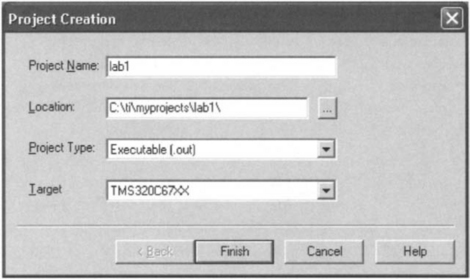
To create a project, choose the menu item Project → New from the CCS menu bar. This brings up the dialog box Project Creation, as shown in Figure 4-19. In the dialog box, navigate to the working folder, throughout the book assumed to be C: i myprojects, and type a project name in the field Project Name. Then, click the button Finish for CCS to create a project file named lab1.prj. All the files necessary to build an application should be added to the project.
CCS provides an integrated editor which allows the creation of source files. Some of the features of the editor are color syntax highlighting, C blocks marking in parentheses and braces, parenthesis/brace matching, control indentions, and find/replace/search capabilities. It is also possible to add files to the project from Windows Explorer using the drag-and-drop approach. An editor window is brought up by choosing the menu item File → New → Source File. For this lab, let’s type the following assembly code into the editor window:
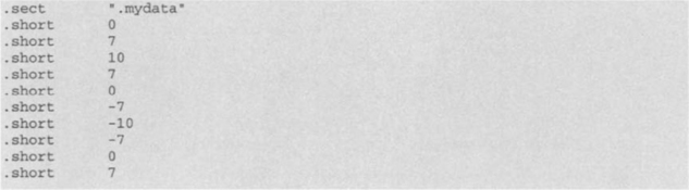
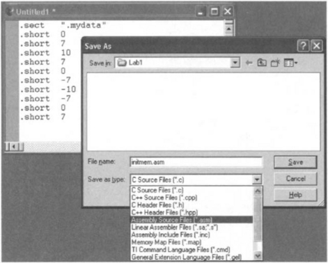
This code consists of the declaration of 10 values using .short directives. Note that any of the data to memory allocation directives can be used to do the same. Assign a section named .mydata to the values by using a .sect directive. Save the created source file by choosing the menu item File → Save. This brings up the dialog box Save As, as shown in Figure 4-20. In the dialog box, go to the field Save as type and select Assembly Source Files (*.asm) from the pull-down list. Then, go to the field File name, and type initmem.asm. Finally, click Save so that the code can be saved into an assembly source file named initmem.asm.
In addition to source files, a linker command file must be specified to create an executable file and to conform to memory specifics of the target DSP on which the executable file is going to run. A linker command file can be created by choosing File → New → Source File. For this lab, let’s type the command file shown in Figure 4-21. This file can also be downloaded from the accompanying CD-ROM. This linker command file is configured based on the DSK memory map. Since our intention is to place the array of values defined in initmem.asm into the memory, a space that will not be overwritten by the compiler should be selected. The external memory space CE0 can be used for this purpose. Let us assemble the data at the memory address 0x8 0000000 (0x denotes hex) located at the beginning of CE0. This is done by assigning the section named .mydata to MYDATA via adding .mydata ≥ MYDATA to the SECTIONS part of the linker command file, as shown in Figure 4-21. Save the editor window into a linker command file by choosing File → Save or by pressing Ctrl + S. This brings up the dialog box Save As. Go to the field Save as type and select TI Command Language Files (*.cmd) from the pull-down list. Then, type lab1. cmd in the field File name and click Save.
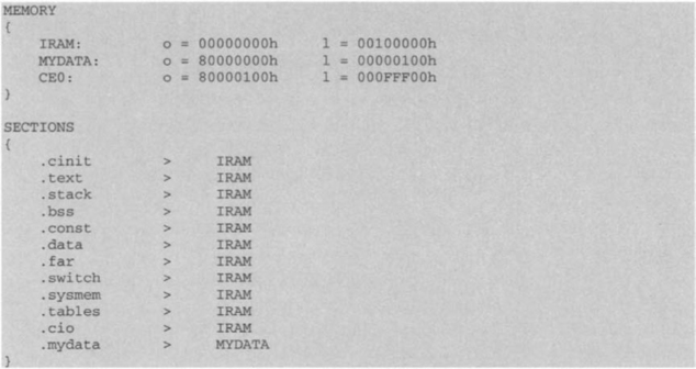
Figure 4-21 Linker command file for Lab 1
Now that the source file initmem.asm and the linker command file lob1.cmd are created, they should be added to the project for assembling and linking. To do this, choose the menu item Project → Add Files to Project. This brings up the dialog box Add Files to Project. In the dialog box, select initmem.asm and click the button Open. This adds initmem.asm to the project. In order to add lob1.cmd, choose Project → Add Files to Project. Then, in the dialog box Add Files to Project, set Files of type to Linker Command File (*.cmd), so that lob1.cmd appears in the dialog box. Now, select lob1.cmd and click the button Open. In addition to initmem.asm and lob1.cmd files, the runtime support library file should be added to the project. To do so, choose Project → Add Files to Project, go to the compiler library folder, here assumed to be the default option C: ic6000cgtoolslib, select Object and Library Files (*.0*,*.l*) in the box Files of type, then select rts6700.lib and click Open. If running on the fixed-point DSP TMS320C6211, select rts6200.lib instead. For debugging purposes, let us use the following empty shell C program. Create a C source file main. c, enter the following lines and add main.c to the project in the same way as just described.
After adding all the source files, the command file and the library file to the project, it is time to either build the project or to create an executable file for the target DSP. To do this, choose the Project → Build menu item. CCS compiles, assembles, and links all of the files in the project. Messages about this process are shown in a panel at the bottom of the CCS window. When the building process is completed without any errors, the executable lab1.out file is generated. It is also possible to do incremental builds – that is rebuilding only those files changed since last build, by choosing the menu item Project → Rebuild. The CCS window provides shortcut buttons for frequently used menu options, such as build ![]() and rebuild all
and rebuild all ![]()
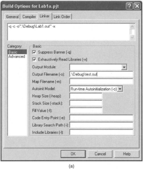
Although CCS provides default build options, these options can be changed by choosing Project → Build Options. For instance, to change the executable filename to test.out, choose Project → Build Options, click the Linker tab of the Build Options window, and type test.out in the field Output Filename (-o), as shown in Figure 4-22a. Notice that the linker command file will include test.out as you click on this window.

All the compiler, assembler, and linker options are set through the menu item Project → Build Options. Among many compiler options shown in 4-22b, pay particular attention to the optimization level options. There are four levels of optimization (0, 1, 2, 3), which control the type and degree of optimization. Level 0 optimization option performs control-flow-graph simplification, allocates variables to registers, eliminates unused code, and simplifies expressions and statements. Level 1 optimization performs all Level 0 optimizations, removes unused assignments, and eliminates local common expressions. Level 2 optimization performs all Level 1 optimizations, plus software pipelining, loop optimizations, and loop unrolling. It also eliminates global common subexpressions and unused assignments. Finally, Level 3 optimization performs all Level 2 optimizations, removes all functions that are never called, and simplifies functions with return values that are never used. It also inlines calls to small functions and reorders function declarations.
Note that in some cases, debugging is not possible due to optimization. Thus, it is recommended to first debug your program to make sure that it is logically correct before performing any optimization. Another important compiler option is the Target Version option. When the application is for the floating-point target DSP TMS320C6711/6713 DSK, go to the Target Version field and select 671x (-mV 6710) from the pull-down list. For the fixed-point target DSP TMS320C6416 DSK, select C64xx (–mv 6400). For the EVM target TMS320C6701, select C670x.
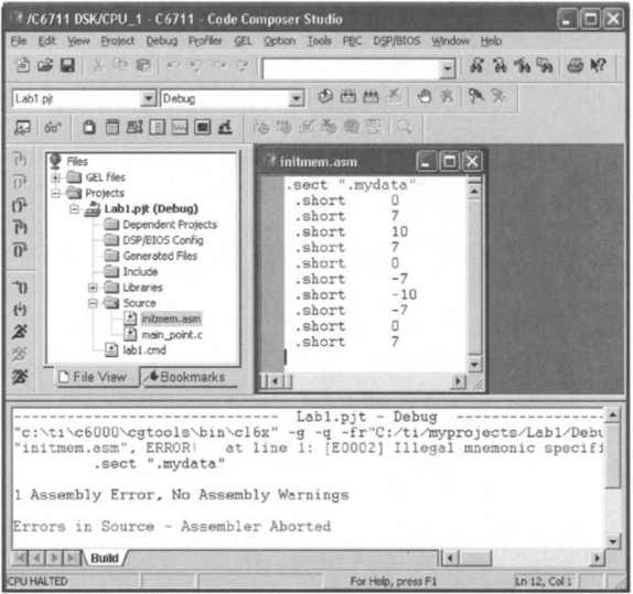
One common mistake in writing initmem.asm is to type directives .sect and .short in the first column. Because only labels can start in the first column, this will result in an assembler error. When a message stating a compilation error appears, click Stop Build and scroll up in the Build area to see the syntax error message. Doubleclick on the red text that describes the location of the syntax error. Notice that the initmem.asm file opens, and your cursor appears on the line that has caused the error, see Figure 4-23. After correcting the syntax error, the file should be saved and the project rebuilt.
L1.2 Debugging Tools
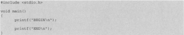
Once the build process is completed without any errors, the program can be loaded and executed on the target DSP. To load the program, choose File → Load Program, select the program lab1.out just rebuilt, and click Open. To run the program, choose the menu item Debug → Run. You should be able to see BEGIN and END appearing in the Stdout window.
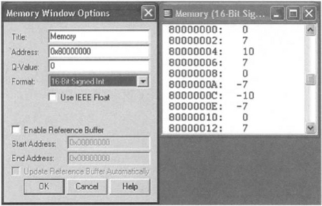
Now, let us verify if the array of values is assembled into the specified memory location. CCS allows one to view the content of memory at a specific location. To view the content of memory at 0x80000000, select View → Memory from the menu. The dialog box Memory Window Options will appear. This dialog box allows one to specify various attributes of the Memory window. Go to the Address field and enter 0x80000000. Then, select 16-bit Signed Int from the pull-down list in the Format field and click OK. A Memory window appears as shown in Figure 4-24. The contents of CPU, peripheral, DMA, and serial port registers can also be viewed by selecting View → Registers → Core Registers, for example.
There is another way to load data from a PC file to the DSP memory. CCS provides a probe point capability, so that a stream of data can be moved from the PC host file to the DSP or vice versa. In order to use this capability, a Probe Point should be set within the program by placing the mouse cursor at the line where a stream of data needs to be transferred and clicking the button Probe Point ![]() . Then, choose File → File I/0 to invoke the dialog box File I/0. Click the button Add File and select the data file to load. Now the file should be connected to the probe point by clicking the button Add Probe Point. In the Probe Point field, select the probe point to make it active, then connect the probe point to the PC file through File In: … in the field Connect To. Click the button Replace and then the button OK. Finally, enter the memory location in the Address field and the number of data in the Length field. Note that a global variable name can be used in the Address field. The probe point capability is frequently used to simulate the execution of an application program in the absence of any live signals. A valid PC file should have the correct file header and extension. The file header should conform to the following format:
. Then, choose File → File I/0 to invoke the dialog box File I/0. Click the button Add File and select the data file to load. Now the file should be connected to the probe point by clicking the button Add Probe Point. In the Probe Point field, select the probe point to make it active, then connect the probe point to the PC file through File In: … in the field Connect To. Click the button Replace and then the button OK. Finally, enter the memory location in the Address field and the number of data in the Length field. Note that a global variable name can be used in the Address field. The probe point capability is frequently used to simulate the execution of an application program in the absence of any live signals. A valid PC file should have the correct file header and extension. The file header should conform to the following format:
![]()
MagicNumber is fixed at 1651. Format indicates the format of samples in the file: 1 for hexadecimal, 2 for integer, 3 for long, and 4 for float. StartingAddress and PageNum are determined by CCS when a stream of data is saved into a PC file. Length indicates the number of samples in the memory. A valid data file should have the extension .dat.
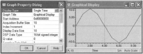
A graphical display of data often provides better feedback about the behavior of a program. CCS provides a signal analysis interface to monitor a signal or data. Let us display the array of values at 0x8 0000000 as a signal or a time graph. To do so, select View → Graph → Time/Frequency to view the Graph Property Dialog box. Field names appear in the left column. Go to the Start Address field, click it and type 0x80000000. Then, go to the Acquisition Buffer Size field, click it and enter 10. Finally, click on DSP Data Type, select 16-bit signed integer from the pull-down list, and click OK. A graph window appears with the properties selected. This is illustrated in Figure 4-25. You can change any of these parameters from the graph window by right-clicking the mouse, selecting Properties, and adjusting the properties as needed. The properties can be updated at any time during the debugging process.
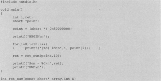
To assign a pointer to the beginning of the assembled memory space, the memory address can be typed in directly to a pointer. It is necessary to typecast the pointer to short since the values are of that type. The following code can be used to assign a pointer to the beginning of the values and loop through them to print each onto the Stdout window:
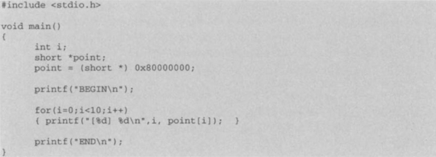
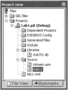
Instead of creating a new source file, we can modify the existing main.c by double-clicking on the main.c file in the Project View panel, as shown in Figure 4-26. This action will bring up the main.c source file in the right-half part of the CCS window. Then, enter the code and rebuild it. Before running the executable file, make sure you reload the file lob1.out. By running this file, you should be able to see the values in the Stdout window. Double-clicking in the Project View panel provides an easy way to bring up any source or command file for reviewing or modifying purposes.
When developing and testing programs, one often needs to check the value of a variable during program execution. This can be achieved by using breakpoints and watch windows. To view the values of the pointer in main.c before and after the pointer assignment, choose File → Reload Program to reload the program. Then, double-click on main.c in the Project View panel. You may wish to make the window larger so that you can see more of the file in one place. Next, put your cursor on the line that says point = (short *) 0x80000000 and press F9 to set a breakpoint. To open a watch window, choose View → Watch Window from the menu bar. This will bring up a Watch Window with local variables listed in the Watch Locals tab. To add a new expression to the Watch Window, select the Watch 1 tab, then type point (or any expression you desire to examine) in the Name column. Then, choose Debug → Run or press F5. The program stops at the breakpoint and the Watch Window displays the value of the pointer. This is the value before the pointer is set to 0x80000000. By pressing F10 to step over the line, or the shortcut button ![]() , you should be able to see the value 0x80000000 in the Watch Window.
, you should be able to see the value 0x80000000 in the Watch Window.
To add a simple C function that sums the values, we can simply pass the pointer to the array and have a return type of integer. For the time being, what is of concern is not how the variables are passed, but rather how much time it takes to perform the operation.
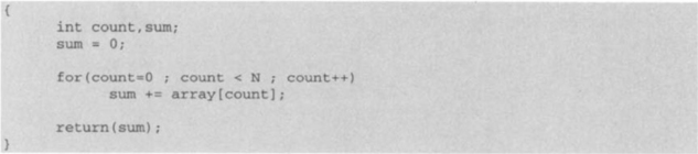
The following simple function can be used to sum the values and return the result:
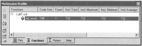
As part of the debugging process, it is normally required to benchmark or time the application program. In this lab, let us determine how much time it takes for the function ret_sum ( ) to run. To achieve this benchmarking, reload the program and choose Profiler → Start New Session. This will bring up Profile Session Name. Type a session name, MySession by default, then click OK. The Profile window showing code size and statistics about the number of cycles will be docked at the bottom of CCS. Resize this window by dragging its edges or undock it so that you can see all the columns. Now right-click on the code inside the function to be benchmarked, then choose Profile Function → in … Session. The name of the function will be added to the list in the Profile window. Finally, press F5 to run the program. Examine the number of cycles shown in Figure 4-27 for ret_sum ( ). It should be about 732 cycles (the exact number may slightly vary). This is the number of cycles it takes to execute the function ret_sum ( ).
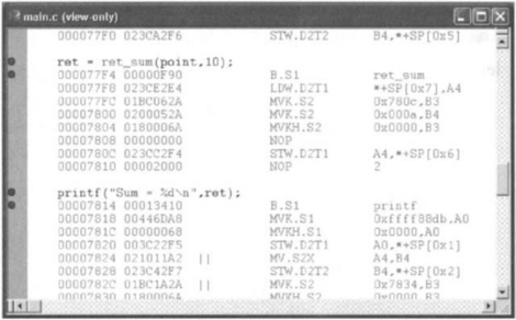
There is another way to benchmark codes using breakpoints. Double-click on the file main.c in the Project View panel and choose View → Mixed Source/ASM to list the assembled instructions corresponding to C code lines. Set a breakpoint at the calling line by placing the cursor on the line that reads ret = ret_sum (point, 10), then press F9 or double-click Selection Margin located on the left-hand side of the editor. Set another breakpoint at the next line as indicated in Figure 4-28. Once the breakpoints are set, choose Profiler → Enable Clock to enable the profile clock. Then, choose Profiler → View Clock to bring up a window displaying Profile Clock. Now, press F5 to run the program. When the program is stopped at the first breakpoint, reset the clock by double-clicking the inner area of the Profile Clock window. Finally, click Step Out or Run in the Debug menu to execute and stop at the second breakpoint. Examine the number of clocks in the Profile Clock window. It should read 752. The discrepancy between the breakpoint and the profile approaches is originated from the extra procedures for calling functions, for example, passing arguments to function, storing return address, branching back from function, and so forth.
A workspace containing breakpoints, probe points, graphs, and watch windows, can be stored for recalling purposes. To do so, choose File → Workspace → Save Workspace As. This will bring up the Save Work window. Type the workspace name in the File name field, then click Save.
The file shown next is an assembly program for calculating the sum of the values. Here, the two arguments of the sum function are passed in registers A4 and B4. The return value gets stored in A4 and the return address in B3. The order in which the registers are chosen is governed by the passing argument convention discussed later. The name of the function should be preceded by an underscore as .global _sum. Create a new source file sum.asm, as shown next, and add it to the project so that main ( ) can call the function sum ( ).
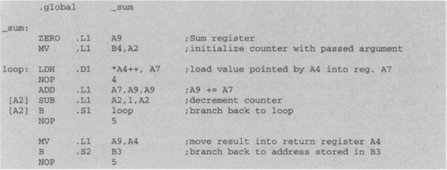
To save the file, go to the Save as type field and select Assembly Source Files (*.asm) from the pull-down list.
The program main ( ) must also be modified by adding a function call to the assembly function sum ( ). This program is shown in Figure 4-29. Build the program and run it. You should be able to see the same return value.
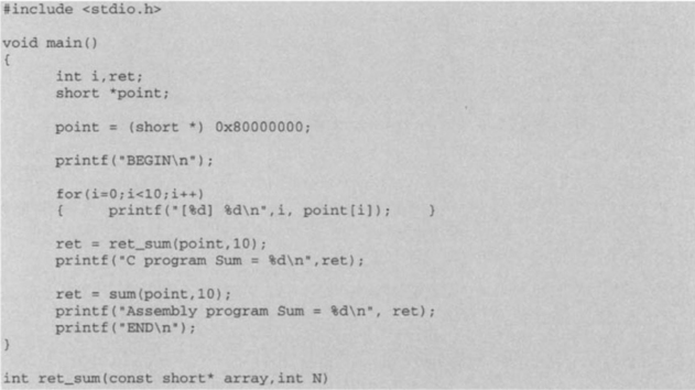
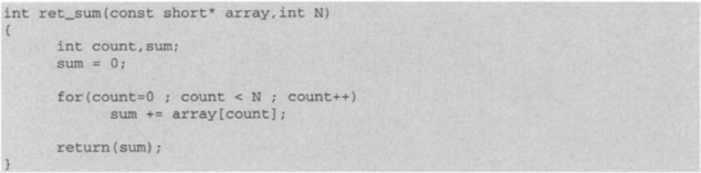
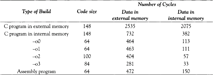
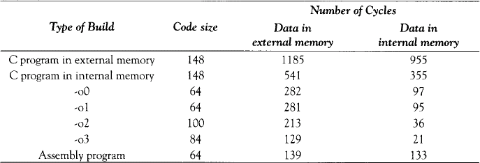
Table 4-2 provides the number of cycles it takes to run the sum function using several different builds. When a program is too big to fit into the internal memory, it has to be placed into the external memory. Although the program in this lab is small enough to fit in the internal memory, it is placed in the external memory to study the change in the number of cycles. To move the program into the external memory, open the lab1.cmd file and replace the line .text ≥ IRAM with .text ≥ CEO. As seen in Table 4-2, this build slows down the execution to 2535 cycles. In the second build, the program resides in the internal memory and the number of cycles is hence reduced to 732. By increasing the optimization level, the number of cycles can be further decreased to 281. The assembly version of the program gives 472 cycles. This is slower than the fully optimized C program because it is not yet optimized. Optimization of assembly codes will be discussed later. At this point, it is worth pointing out that, throughout the labs, the stated numbers of cycles indicate timings on the C6711 DSK with CCS version 2.2. The numbers of cycles will vary slightly depending on the DSK target and CCS version used.
L1.3 EVM Target
As described in Section 4.1 and illustrated in Figure 4-7, the memory map of EVM possesses more internal/external memory space than that of DSK, thus allowing more flexibility in loading code into the program/data section. Figure 4-30 shows an example using the EVM target where data located at EXT3, say 0x03000000, is placed at the beginning of EXT3.
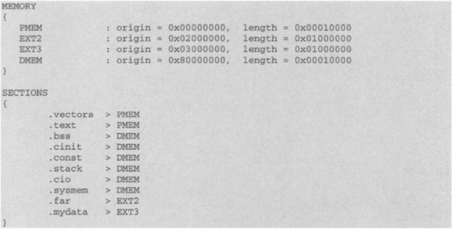
Figure 4-30 Command file for Lab 1
In order to place the program code into the external memory, replace the line .text ≥ PMEM with .text ≥ EXT2. The number of cycles on the EVM target is shown in Table 4-3. To build the project, the library rts6701.lib for C6701 EVM or rts6201.lib for C6201 EVM needs to be added into the project. The Target Version field of the Build option should be selected as C670x (-mv 6700) for the floating-point target DSP TMS320C6701 EVM or C620x (-mv 6200) for the fixed-point target DSP TMS320C6201 EVM.
As a final note, it is worthwhile to mention a remark about the EVM board resetting. Sometimes you may notice that your program cannot be loaded into the DSP even though there is nothing wrong with it. Under such circumstances, you need to reset the EVM board to fix the problem. However, you have to close CCS before you reset the board. Otherwise, the problem will not be resolved.
L1.4 Simulator
When no DSP board is available, the CCS simulator can be used to run the lab programs. To configure CCS as a simulator, simply select simulator in the field Platform during the installation process of CCS, as shown in Figure 4-31. In the Import Configurations window, select the simulator option for one of the specified DSP boards. By clicking the button Import, then the button Save and Quit, the simulator gets configured and becomes ready to use. Note that although the simulator supports DMA and EMIF operations, operations related to McBSP, HPI and Timer are not supported. The files for running the labs via the simulator are provided under the simulator folder on the accompanying CD-ROM.
