Real-Time Analysis and Scheduling
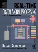
Figure 10-1 provides an overview of the conventional CCS debugging techniques based on breakpoints, probe points, and profiler. Although these debugging tools are very useful to see whether an application program is logically correct or not, when it comes to making sure that real-time deadlines are met, they have limitations. The so-called DSP/BIOS feature of CCS complements the traditional debugging techniques by providing mechanisms to analyze an application program as it runs on the target DSP without stopping the processor. In traditional debugging, the target DSP is normally stopped and a snap shot of the DSP state is examined. This is not an effective way to test for real-time glitches.
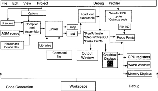
DSP/BIOS consists of a number of software modules that get glued to an application program to provide real-time analysis and scheduling capabilities. A listing of all available modules is provided in Figure 10-2. CCS provides an easy-to-use way to glue these modules to the application program. Figure 10-3 shows a sample C file with a BIOS object, a BIOS function, and its corresponding section names. The size of the DSP/BIOS portion of an application program is limited to a maximum of 2K words and is proportional to the number of modules and objects used.

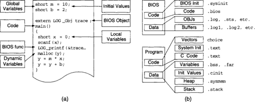
Figure 10-4 shows a listing of the DSP/BIOS modules accessed by the Configuration Tool feature of CCS. This figure also shows the files generated by the Configuration Tool. The Configuration Tool is a visual editor which allows one to create module objects and set their properties. An application program can interact with objects by using DSP/BIOS API functions. In addition, DSP/BIOS plug-ins can be activated from the CCS environment, providing real-time instrumentation including log and statistics displays.
Figure 10-5 illustrates all the files created within the CCS environment when using DSP/BIOS; the files with white background are created by the user and the ones with grey background by CCS. The naming convention used by the modules is shown in Figure 10-6. The datatypes associated with a module are defined in its header file. Header files of those modules which are used in real-time analysis of an application program must be included in the program.
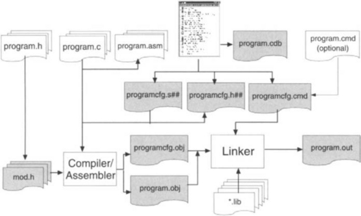
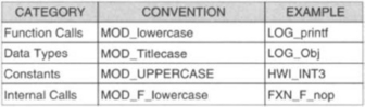
Figure 10-6 Three letter prefix module naming conventions, capitalization convention distinguishes functions, types, and constants.
In essence, DSP/BIOS provides real-time analysis, real-time scheduling, and realtime data exchange capabilities for debugging application programs. As a result, one can make sure that an application program is meeting its real-time deadlines in addition to being logically correct.
10.1 Real-Time Analysis
There are two types of real-time constraints: (a) hard real-time, denoting critical real-time needs (i.e., timing needs that should be met to avoid system failure), and (b) soft real-time, denoting not-so-critical real-time needs that can be done as time becomes available. For example, as shown in Figure 10-7, the response to incoming samples must be done in a hard real-time manner in order not to lose any information, whereas data transfer from the target DSP to the host can be done in soft real-time.
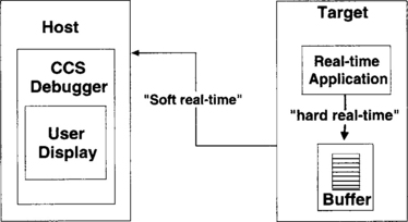
Figure 10-7 Hard and soft real-time: data buffered in hard real-time, and sent to host in soft real-time.
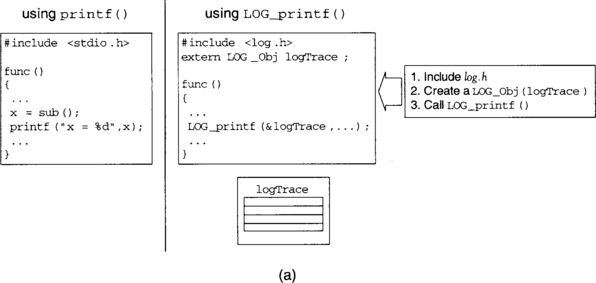
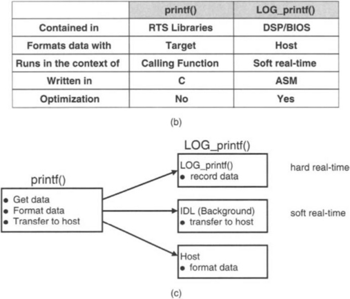
To monitor the status of a program in real-time, it is possible to use the C function printf ( ) as defined in the real-time support library. However, this function takes too many cycles to run, an undesirable property as far as real-time performance is concerned. On the other hand, LOG_printf ( ) is a LOG module API that creates a buffer. The buffer is then sent to the host in soft real-time. The buffer size n is specified as part of a LOG object. A LOG object can be configured in fixed or circular mode. The fixed mode captures the first n occurrences, while the circular mode captures the last n occurrences. LOG_printf ( ) runs in much fewer clock cycles as compared with print ( ). Figures 10-8(a), 10-8(b), and 10-8(c) illustrate the difference between printf ( ) and LOG_printf ( ).
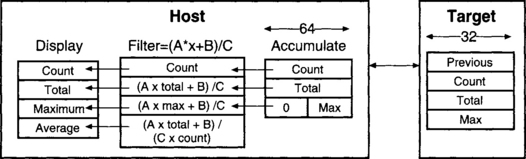
Statistics on a value can be captured by using the STS_add ( ) API. Two other statistics API, STS_set ( ) and STS_delta ( ), can be used to time a piece of code. The plug-in Statistics View window can be activated on the host as part of CCS to monitor the statistics associated with a variable. These statistics are reconfigured on the host as shown in Figure 10-9.
The trace module through the RTA Control Panel of DSP/BIOS allows various modules to be enabled or turned on so that only a specific or needed portion of the DSP/BIOS kernel is glued to the application program. The RTA Control Panel properties can be set to decide how often the host should poll the target DSP for various logging and statistics data. The CPU Load Graph is another plug-in instrumentation which shows the monitoring of the CPU active time as a program runs on the target DSP.
10.2 Real-Time Scheduling
This is done by breaking down the application program into threads each doing a specific function or task. Some of the threads may occur more often than others. Some of them may be subject to hard real-time and some to soft real-time constraints. The real-time need of the entire application program or system is met by appropriately prioritizing threads. This multithreaded real-time scheduling approach is what makes it possible to meet real-time timing deadlines.
Threads can be scheduled using hardware interrupts (ISRs) in a non-preemptive fashion by disabling hardware interrupts. The scheduling can be done in a preemptive fashion by prioritizing hardware interrupts. Considering that not all real-time situations can be handled by preemptive hardware interrupts, a more robust scheduling mechanism based on software interrupts is adopted in DSP/BIOS. Software interrupts automatically perform context switching (i.e., storage/retrieval of the DSP status to the time the interrupt occurred).
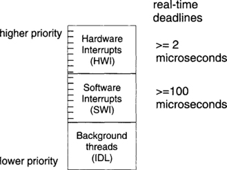
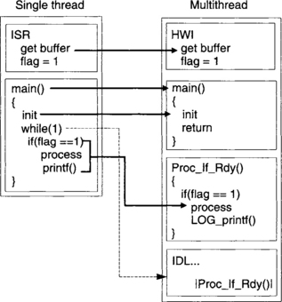
DSP/BIOS uses a background/foreground scheduling approach where the background consists of non-critical housekeeping threads such as transferring information to the host and instrumentation. These threads or functions are done in a round-robin fashion as part of idle or background loop IDL. The foreground consists of more critical threads. These threads are implemented via hardware (HWI module) and software (SWI module) interrupts. Hardware interrupts have higher priority than software interrupts. As indicated in Figure 10-10, normally software interrupts are used for deadlines of 100 microsec or more, and hardware interrupts for more restrictive deadlines of 2 microsec or more. The priority of software interrupts can easily be changed through SWI objects. Software interrupts can be posted unconditionally or conditionally via mailboxes. In essence, the DSP/BIOS scheduling is based on preemptive software interrupts. Figure 10-11 shows an example of how a single-thread ISR is converted to a hardware, software, and idle multithread program. In addition to hardware and software threads, the upgraded version of DSP/BIOS provides a task TSK module which can be used for posting threads capable of yielding to other threads.
There are basically two thread scheduling rules. The first rule is that if a higher priority thread becomes ready, the running thread is preempted. The second rule is that threads having the same priority are scheduled in a first-in first-out fashion. Three examples are shown in Figure 10-12 to illustrate how various threads run based on the scheduling rules. In this figure, a running thread is shown by shaded blocks and a thread in ready state by white blocks per time tick. The Execution Graph window feature of DSP/BIOS provides a visual display of execution of threads. It shows which thread is running and which threads are in ready state. It also provides useful feedback information on errors. Errors are generated when real-time deadlines are missed or when the system log is corrupted. An example of the Execution Graph window is shown in Figure 10-13. It should be noted that in the Execution Graph window, although time intervals between time ticks are the same, they may not be displayed as equal. This provides a more compact way to show all events between two successive time ticks.
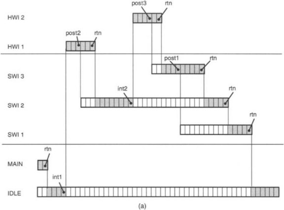
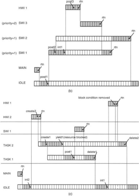
Figure 10-12 Examples of threads running based on scheduling rules, gray blocks indicate running status and white blocks ready status.†
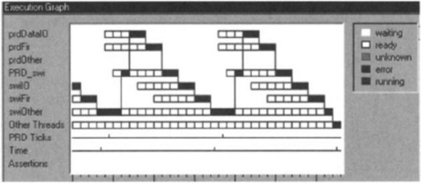
There are two timers on the C6x, each is controlled by three memory-mapped registers: the Timer Control Register for setting the operating mode, the Timer Period Register for holding the number of clock cycles to count, and the Timer Counter Register for holding the current clock cycle count. As illustrated in Figure 10-14, the clock module CLK is used to set the on-chip timer registers for low (determined by the Timer Period Register) or high resolution (the CPU clock divided by 4) ticks. The clock APIs run as hardware functions. The PRD module is used to run threads that are to be executed periodically. The period is specified as part of a PRD object. The period APIs run as software functions. The CLK manager is used to drive the PRD module.
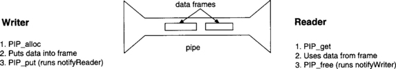
Data frame synchronization and communication can be achieved by using the PIP module. A pipe consists of a specified number of frames having a specified size. It has two ends, a writer end and a reader end. The sequence of operations on the writer side consists of getting a free frame from the pipe via PIP_alloc ( ), writing to it, and putting it back in the pipe via PIP_put ( ), which runs the notifyReader ( ) function. The sequence of operations on the reader side consists of getting a full frame from the pipe via PIP_get ( ), reading it, and putting the empty frame in the pipe via PIP_free ( ), which runs the notifyWriter ( ) function. Figure 10-15 illustrates this process.
10.3 Real-Time Data Exchange
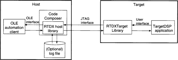
The RTDX (Real-Time Data Exchange) module can be used to exchange data between the DSP and the host without stopping the DSP. Similar to other modules, this exchange of information between the host and the DSP is done via the JTAG (Joint Test Action Group) connection, an industry-standard connection. The RTDX module provides a useful tool when values need to be modified on the fly as the DSP is running. As shown in Figure 10-16, RTDX consists of both target and host components, each running its own library. On the host side, various displays and analysis OLE (object linking and embedding) automation clients, such as LabVIEW, Visual Basic, Visual C++, can be used to display and send data to the application program. RTDX can be configured in two modes: non-continuous and continuous. In non-continuous mode, data is written to a log file on the host. This mode is normally used for recording purposes. In continuous mode, the data is buffered by the RTDX host library. This mode is normally used for continuously displaying data.
Labs 7 and 8 that follow provide a hands-on experience with the DSP/BIOS features of CCS. Lab 7 covers its real-time analysis and scheduling and Lab 8 its data synchronization and communication aspects. More details on the DSP/BIOS modules can be found in the TMS320C6000 DSP/BIOS User’s Guide manual [1].
Lab. 7 DSP/BIOS
The objective of this lab is to become familiar with the DSP/BIOS feature of CCS. DSP/BIOS includes a real-time library which allows one to interact with an application program in real-time as it runs on the target DSP. To build a program based on DSP/BIOS, the Configuration Tool feature of CCS needs to be used to create objects and set their properties. The Configuration Tool is opened by choosing the menu item File → New → DSP/BIOS Configuration. The configuration of a program can be saved via File → Save, and Configuration Files (*.cdb) in the Save as type drop-down box. A saved configuration file includes all the necessary files for generating an executable file.
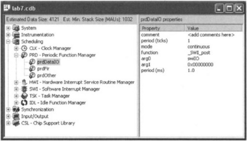
A DSP/BIOS object can be created by right-clicking on a module displayed in the Configuration Tool window and by selecting Insert. For example, as shown in Figure 10-17, to create a PRD object, right-click on PRD – Periodic Function Manager and select Insert PRD. This adds a new object for the PRD module. An object can be renamed by right-clicking on its name and choosing Rename from the pop-up menu. Properties of an object can be displayed by right-clicking on the object icon and selecting Properties from the pop-up menu. From the property sheet, property settings can be readily changed.
L7.1 A DSP/BIOS-Based Program
The following C code is an example of a simple DSP/BIOS-based program. This program compares the performance of the DSP/BIOS API LOG_printf ( ) to the function printf ( ), which is a part of the run-time support library:
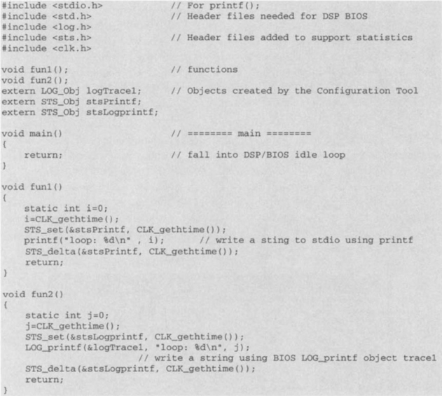
Two functions are declared in this program: fun1 ( ) and fun2 ( ), one using printf ( ) and the other LOG_printf ( ). These functions obtain the processing time and print them on the screen. Printing is the most widely used way to view results of a program. As shown in Figure 10-8, LOG_jorintf ( ) is optimized to take much fewer instruction cycles than printf ( ). It sends buffered data to the host in soft real-time to avoid missing real-time deadlines. On the other hand, printf ( ) does not use the background scheduling approach for transferring data to the host and, hence, may cause the program to miss its real-time deadlines. At this point, it is worth mentioning that although it is possible to use Watch Window, this option interrupts the DSP in order to transfer data and does not meet the real-time requirement.
Note that appropriate header files should be included to build a DSP/BIOS-based program. Foremost, the header file std .h should be included whenever using any DSP/BIOS API. The header files, log.h, sts.h, and clk.h, corresponding to the three modules LOG, STS, and CLK, respectively, are included in the aforementioned program. Any created DSP/BIOS objects should also be declared. There are three declared objects here: logTracel, stsPrintf, and stsLogprintf. The LOG object logTracel managed by the LOG module allows real-time logging. The STS objects managed by the STS module store key statistics in real-time. The STS_set ( ) and STS_delta ( ) APIs use the information stored in the STS objects to compute the required number of instruction cycles to run printf ( ) or LOG_printf ( ).
Now let us create the objects declared in the program. First, a configuration file is created by choosing File → New → DSP/BIOS Configurations. If a configuration file already exists, it can be activated by double-clicking on it in the Project View panel. To add a LOG object as part of the LOG_printf ( ) API, right-click on LOG-Event Log manager in the Configuration Tool and select the option Insert LOG from the pop-up menu. This causes LOGO to be inserted. Since the name logTracel is used here, rename this object by right-clicking on it and then by selecting Rename. Change the name to logTracel. Right-click on logTracel to change its properties. Select Cancel noting that the default settings are fine for this lab. Next, create two STS objects in a similar manner and rename them as stsPrintf and stsLogprintf. The properties of these objects will be discussed in the next section. Use File → Save to save the configuration file.
L7.2 DSP/BIOS Analysis and Instrumentation
Real-time analysis allows one to determine whether an application program is operating within its real-time deadlines and whether its timing can be improved. DSP/BIOS instrumentation APIs and DSP/BIOS plug-ins enable real-time data gathering and monitoring as an application program is running. For example, when using the instrumentation API LOG_printf ( ), the communication between the DSP and the host is performed during the idle state or in the background. The idle thread has the lowest priority. As a result, the real-time behavior of an application program is not affected.
In the preceding program, the instrumentation APIs STS_set ( ) and STS_delta ( ) are used to benchmark the functions printf ( ) and LOG_printf ( ). STS_set ( ) saves the value specified by CLK_gethtime ( ) as the previous value in the STS object. STS_delta ( ) subtracts this saved value from the value it is passed. Consequently, STS_delta ( ) in conjunction with STS_set ( ) provide the difference between the start and completion of the function in between. However, to obtain an accurate benchmarking outcome, the overhead associated with the instrumentation APIs should be subtracted. To calculate this overhead, the program should be run again by leaving out LOG_printf ( ) and printf ( ).
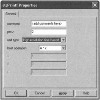
Before calculating the overhead, let us examine how the STS objects should be used during benchmarking. Since the STS objects count system ticks, they do not provide the actual CPU instruction cycles. A filtering operation on the host is normally performed to show the actual CPU instruction cycles. This is done by changing the properties of the STS objects via right-clicking and selecting Properties from the pop-up menu. In the properties box, go to the unit type field and choose High resolution time based from the drop-down menu. This changes the host operation field to A*x and the value in the A field to 4, as shown in Figure 10-18.
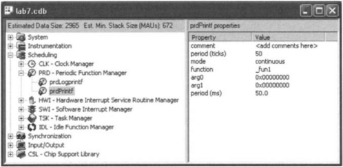
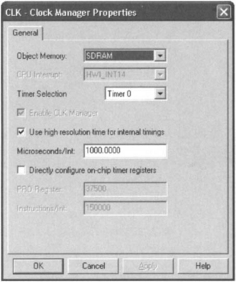
One mechanism to come out of the idle state in main ( ) is to use PRD objects to call fun1 ( ) and fun2 ( ). In this lab, such an approach is adopted by activating PRD objects every 50msec. These objects are created by right-clicking on PRD – Periodic Function Manager and selecting Insert PRD. The objects need to be renamed as prdPrintf and prdLogprintf. For the object prdPrintf, change the properties as illustrated in Figure 10-19. Since the property period(ticks) is set to 50, this object calls the function mentioned in the property field function every 50 msec. This is because 1 tick (or timer interrupt) is set to 1000 microsec (or 1 msec) in the CLK – Clock Manager module. The property of this module is changed by right-clicking on CLK – Clock Manager and selecting Property, as shown in Figure 10-20. Notice that when specifying the function fun1 ( ) in the property field function, an underscore should be added before it. This rule holds for a C function to be run by DSP/BIOS objects. The underscore prefix is necessary because the Configuration Tool creates assembly source, and the C calling convention requires the underscore when calling C from assembly. For the prdLogprintf object, similarly enter _fun2 in the property field function.
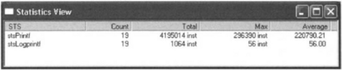
After building the program, in order to view the statistics information captured by the STS objects, choose the menu item DSP/BIOS → Statistics View. Then, right-click in this window and select Property Page. In the Statistics View Dialog Box, click on the objects stsPrintf and stsLogprintf, then click OK. You may wish to resize the window so that all of the statistics can be viewed. Run the program. Without printf ( ) or LOG__printf ( ), the average number of instruction cycles captured by the STS objects are 86 and 92, respectively, which correspond to the overhead for calling STS_set ( ) and STS_delta ( ). Next, rebuild with printf ( ) and LOG_printf ( ). In order to eliminate the overhead, change the properties of the STS objects as follows: host operation = (A * x + B), A = 4 and B = −86 for stsPrintf and B = −92 for stsLogprintf. Run the program again. The Statistics View window displays 220790 instruction cycles for printf ( ) and 56 for LOG_printf ( ), as shown in Figure 10-21.
The output of LOG_printf ( ) can be seen via a message log window. Select the menu item DSP/BIOS → Message Log. A new window will appear. This window should then be linked to the LOG object. In the drop-down box Log Name of the Message Log window, select logTracel.
L7.3 Multithread Scheduling
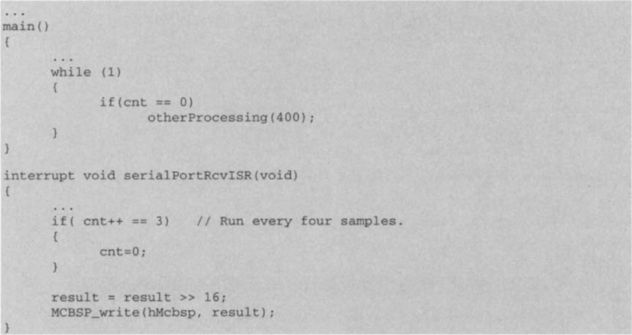
Real-time scheduling involves breaking a program into multiple threads in order to meet a specified real-time throughput. The Lab 4 program is used here to study the real-time scheduling issues. First, the ISR in Lab 4 is modified as follows:
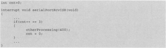
The function otherProcessing ( ) does no specific processing and merely consumes CPU time. This function is shown next:
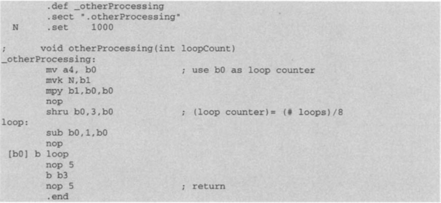
This function sets up a counter using the value passed to it. Let this value be 400. The counter is decreased one at a time in a loop, thus consuming CPU time. This function, of course, can be replaced with an actual processing code.
After building the project, connect the function generator and oscilloscope to the DSK board. Then, run the program. It is observed that the ISR does not meet real-time deadlines due to the extra processing required by the function otherProcessing ( ). In other words, the ISR misses input samples and fails to produce the desired output signal.
Now, let us perform real-time scheduling by breaking up the ISR into three functions or threads, datalo ( ), fir ( ), and otherProcessing ( ), as follows:
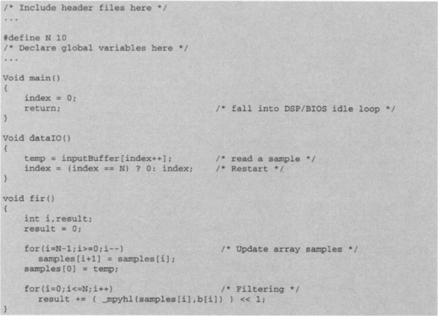
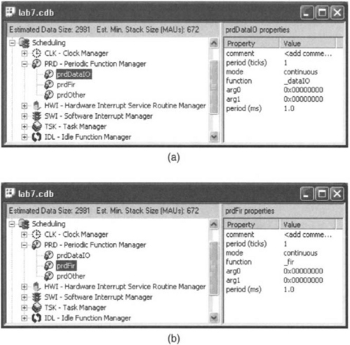
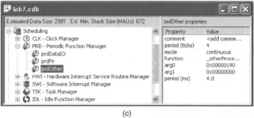
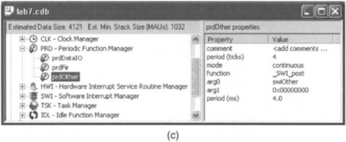
The thread dataIO ( ) reads one sample from inputBuffer whenever it is called. This thread simulates the operation of the MCBSP_read ( ) API. The thread fir ( ) performs FIR filtering. Let us now use three PRD objects to run these threads. Since otherProcessing ( ) is called after every three input samples, it is not necessary to run all three threads or functions at the same period tick. The prdDataIO object runs the function dataIO ( ), and prdFir object runs the function fir ( ) every 1 msec. The prdOther object runs the function otherProcessing ( ) every 4 msec. The property settings of these PRD objects are shown in Figure 10-22.
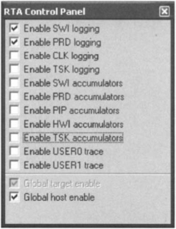
After building the project, to see whether the threads meet their real-time deadlines, choose DSP/BIOS → RTA Control Panel and place check marks in the boxes as indicated in Figure 10-23. Also, enable the global tracing option. Then, invoke the Execution Graph by choosing DSP/BIOS → Execution Graph. Right-click on the RTA Control Panel and choose Property Page from the pop-up menu. Run the program. The Execution Graph should look like the one shown in Figure 10-24.
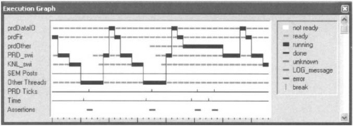
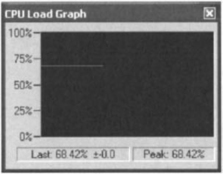
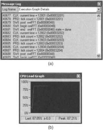
Any missed deadline error appears in the Assertions row of the Execution Graph. From Figure 10-24, it can be seen that there are such errors in the preceding multithread program. Another way to see the same information is via the message log window Execution Graph Details, by choosing DSP/BIOS → Message Log. In the Log Name field of the window, choose Execution Graph Details and click OK. An Execution Graph Details window should appear as shown in Figure 10-25. The information in this window indicates that prdFir ( ) is missing its real-time deadlines. Figure 10-26 shows the CPU load when the program is running. To invoke this window, choose the menu item DSP/BIOS → CPU Load Graph.

To overcome real-time errors, the scheduling of threads need to be changed by assigning different priorities to them. As shown in Figure 10-25, prdFir ( ) is missing its real-time deadlines. This is due to the fact that periodic functions execute at the same priority level, since they run as part of the same software interrupt PRD_swi. This scheduling problem is overcome by allowing each periodic object to post a software interrupt (SWI) object, which then calls the appropriate thread or function.
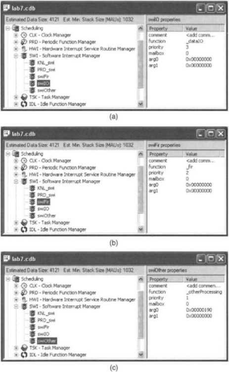
A SWI object has five properties: priority, function, arg0, arg1, and mailbox. The property function causes a specified function to be called when the SWI object is posted. The arguments arg0 and arg1 are passed to the function. The property priority stores the priority level assigned to the SWI object. The mailbox property will be covered in Lab 8. In this lab, three SWI objects are created: swiIO, swiFir, and swiOther. Instead of the PRD objects, the SWI objects are used to run the threads dataIO ( ), fir ( ), and otherProcessing ( ). The swiIO object runs dataIO ( ), the swiFir object runs fir ( ), and the swiOther object runs otherProcessing ( ). Assuming that the real-time constraint of otherProcessing ( ) is not as demanding as dataIO ( ), the priority of swiIO is set to 3 and the priority of swiOther to 1. The property settings of the SWI objects are shown in Figure 10-27.
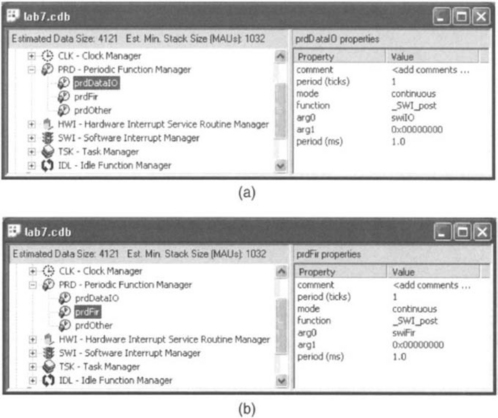
Now that the SWI objects are ready to call the threads or functions, three PRD objects need to be set up to post the software interrupts. This is achieved by changing the properties of the original PRD objects, as shown in Figure 10-28. The PRD_swi thread runs the PRD functions associated with prdDataIO and prdFir every 1 msec and those associated with prdOther every 4 msec. In other words, the PRD functions post the software interrupts associated with the SWI objects. For instance, the prdDataIO object runs the function SWI_post (swiIO), which posts the software interrupt that in turn runs the function dataIO ( ). Although the software interrupts for both swiIO and swiFir are posted every 1 msec, the function dataIO ( ) runs first because the associated swiIO has a higher priority than swiFir. After the dataIO ( ) function completes, the fir ( ) function runs. The software interrupt for swiOther is posted every 4 msec, causing its associated function, otherProcession ( ), to run. However, when a higher priority thread becomes ready, otherProcessing ( ) is preempted. Figure 10-29 shows the scheduling of the periodic and software threads.
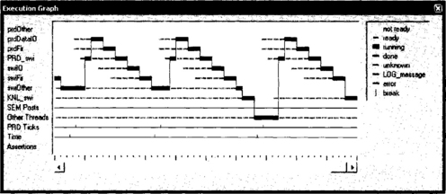
As illustrated in Figure 10-29, no real-time error is observed in the Assertions row because the threads are scheduled in such a way that they all meet their real-time deadlines. In general, critical and frequent events such as sampling should be assigned a higher priority. Next, let us go back to the ISR in the FIR filtering program. Based on the aforementioned real-time scheduling, the otherProcessing ( ) thread can be moved into the while loop in main ( ), since the while loop runs on a lower priority (or in the background). The following piece of code shows this modification:
It can be observed that this program yields the correct FIR filtering output by connecting a function generator and an oscilloscope to the DSK board.
Lab. 8 Data Synchronization and Communication
The objective of this lab is to become familiar with the data synchronization and communication capabilities of DSP/BIOS by using the FFT program discussed in Lab 6. This program uses hardware interrupts to read and process input samples entering the serial port 1 of the DSK, or serial port 0 of the EVM.
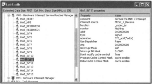
In the DSP/BIOS-based version of this program, the hardware module HWI is used to manage hardware interrupts. Let us use the interrupt INT11 to read input samples from the serial port 1 considering the DSK target. This requires that the properties of the HWI_INT11 object are appropriately set. First, create a new configuration by choosing File → New → DSP/BIOS Configuration. Then, click the + sign next to the HWI – Hardware Interrupt Service Routine manager menu under Instrumentation category, and right-click on HWI_INT11 and select Properties from the pop-up menu. The window HWI INT11 Properties will appear. Select MCSP_l_Receive in the property field interrupt source so that the multichannel buffered serial port 1 is used as the interrupt source. Next, specify the function by entering _codec_isr in the property field function. This function reads a 32-bit input sample from the DRR and stores it into the location indicated by the global pointer rxPtr, which is explained shortly. The source codes of codec_isr ( ) are provided on the accompanying CD-ROM.
Figure 10-30 shows the properties of the HWI_INT11 object. This object is configured to run codec_isr ( ) whenever the hardware interrupt occurs.
The FFT program processes a frame of data when a specified number of samples are collected into an input frame buffer. This program also uses an output frame buffer to send out processed data frames. Since the FFT function should be performed only when the input frame is full and the output frame is empty, the execution of the FFT function needs to be synchronized with the status of the frames. In other words, the FFT function should be aware of whether or not the input frame is full and the output frame is empty. The mailbox property of SWI objects is used here for this purpose.
The mailbox property provides a conditional posting of software interrupts. Only when the mailbox in a SWI object becomes zero is the software interrupt posted by the SWI object. In this lab, a SWI object swiFFT is created and configured to run the FFT function when the mailbox value becomes zero. Initially, the mailbox is set to have a nonzero value of 3 (or 11 in binary). In order to run the FFT function, all the bits in the mailbox should be reset to zero. One possibility is to reset bit 0 to zero when the output frame is empty and reset bit 1 to zero when the input frame is full. The swiFFT object is therefore configured as shown in Figure 10-31. In order to create this object, right-click on SWI – Software Interrupt Manager under the Scheduling category inside the Configuration Tool window and select Insert SWI from the pop-up menu. A SWIO object will be generated. Rename it swiFFT. Change the properties by right-clicking on the swiFFT object and selecting Properties. Inside the dialog box, change the properties as shown in Figure 10-31. The fft ( ) function is assigned to the property function so that it is executed when the mailbox value becomes zero.
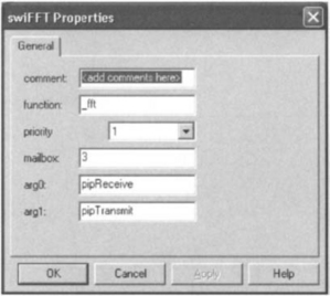
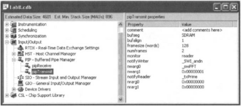
The property settings in Figure 10-31 show that the function fft ( ) takes two arguments: pipReceive and pipTransmit. These are PIP objects, which are used as the input frame and the output frame for the fft ( ) function. The PIP module manages these frames. The interrupt service routine codec_isr ( ) copies data from the DRR to the input frame via the pipRecevice object and from the output frame to the DXR via the pipTransmit object. The PIP objects need to be created and configured so that they can reset appropriate bits in the swiFFT’s mailbox to zero, causing the fft ( ) function to run with a full input frame and an empty output frame. To create the pipReceive object, right-click on PIP – Buffered Pipe Manager under Input/Output category inside the Configuration Tool window, and choose Insert PIP from the pop-up menu. A PIP0 object will be created. Rename it pipReceive by right-clicking on it and selecting Rename. The pipTransmit object is created in the same manner. The properties are then modified to meet the synchronization between the swiFFT and PIP objects. Figure 10-32 shows the properties of the pipReceive object, which is configured to clear bit 1 in the swiFFT’s mailbox when the input frame is full and ready to be processed. To change the properties of the pipReceive object, right-click on it and select Properties from the pop-up menu. A dialog box will appear in which new property values can be entered. The properties of the pipTransmit object are changed in a similar manner.
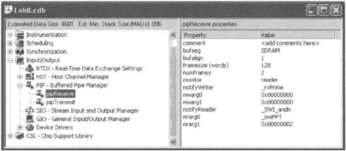
As shown in Figure 10-32, the function _SWI_andn is specified in the property field notifyReader. This property assigns the function to run when the input frame buffer is full and ready to be processed. As a result, whenever the input frame is full, the _SWI_andn function is executed. The _SWI_andn function clears the bits in the mailbox and posts a software interrupt. Its first argument, nrarg0, specifies the SWI object to be applied, and its second argument, nrarg1, denotes the mask. The mailbox value is reset by the bitwise logical AND NOT Operator: mailbox = mailbox AND (NOT mask). Because the pipReceive object has the mask value of 2 (or 10 in binary), it resets bit 1 in the mailbox to zero. Consequently, since swiFFT is the first argument of _SWI_andn, the pipReceive object resets bit 1 of the swiFFT’s mailbox whenever the input frame is full and ready to be processed.
Now that bit 1 of the swiFFT’s mailbox is reset to zero by the pipReceive object, the only condition to run the FFT function is to reset bit 0 considering that 3 (or 11) was the initial value in the mailbox. The pipTransmit object completes the synchronization process. Figure 10-33 shows the properties of the pipTransmit object, which is configured to clear bit 0 of the swiFFT’s mailbox when an empty frame is available. Note that the property field notifyWriter is set to _SWI_andn. This property specifies the function to run when an empty frame is available. Under such a condition, the _SWI_andn function runs with the mask value of 1 (or 01 in binary) and resets bit 0 of the swiFFT’s mailbox to zero. Hence, when the input frame is full and the output frame is empty, pipReceive and pipTransmit reset the swiFFT’s mailbox to zero, causing the FFT function to run.
Next, let us see how the FFT function makes use of data frames in the PIP objects. The following piece of code shows the sequence of events:
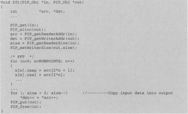
The first argument of the FFT function, in, is the pipReceive object and the second argument, out, is the pipTransmit object, as indicated in Figure 10-31. In order to use the frames in the PIP objects, first the PIP_get ( ) and PIP_alloc ( ) API functions should be called. The PIP_get ( ) API gets a full frame from the pipRecevie object and the PIP_alloc ( ) API allocates an empty frame from the pipTransmit object. Normally, the PIP_get ( ) API is followed by the PIP_getReaderAddr ( ) API, which returns the address for the reading process. Similarly, the PIP_alloc ( ) API is followed by the PIP_getWriterAddr ( ) API, which returns the address for the writing process. A pointer src is therefore used to read from the input frame and a pointer dst to write to the output frame. In this program, the FFT function processes the data stored in src. Before leaving the fft ( ) function, the PIP_put ( ) API is called to put the full frame into the pipTransmit object. Normally, this API is used together with the PIP_alloc ( ) API because PIP_put () puts a frame allocated by PIP_alloc ( ) into a PIP object after the frame is full. Similarly, the PIP_free ( ) API is used together with the PIP_get ( ) API because PIP_free ( ) releases the frame for PIP_get ( ) after it is read. The released frame is recycled so that it can be reused by the PIP_alloc ( ) API.
Note that the value of the property notifyWriter in the pipReceive object is set to _rxPrime, as shown in Figure 10-32. Therefore, the function rxPrime ( ) is called when a frame of free space is available in the pipReceive object. The following piece of code shows the relevant part in the rxPrime ( ) function:
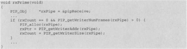
The global variable rxCount keeps track of the remaining number of words for filling up the current rxPipe (or pipReceive) frame. In the codec_isr ( ) function, rxCount is decreased by one whenever a sample is read from the DRR and copied into the rxPipe frame. When this frame becomes full and ready to be put into rxPipe, rxCount becomes zero. Then, this function allocates the next empty frame from rxPipe by calling PIP_alloc (rxPipe). The address of the frame is set to the global variable rxPtr so that codec_isr ( ) can copy the content of the DRR into rxPtr by calling PIP_getWriterAddr (rxPipe). In the codec_isr ( ) function, rxPtr is increased by one to point to the next location whenever the DRR content is copied.
As shown in Figure 10-33, _txPrime is written in the property field notifyReader. Therefore, the function txPrime ( ) runs when a frame is full and ready to be used. The following piece of code shows the relevant part in the txPrime ( ) function:
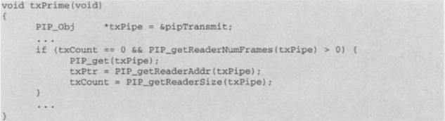
The global variable txCount keeps track of the remaining number of words for transmitting the current txPipe (or pipTransmit) frame. In the function codec_isr ( ), txCount is decreased by one whenever a sample is copied from the txPipe frame and written to the DXR. When all the samples in this frame are written, txCount becomes zero. Then, this function gets the next full frame from txPipe by calling PIP_get (txPipe). The address of the frame is set to the global variable txPtr by calling PIP_getReaderAddr (txPipe) so that codec_isr ( ) can copy the content of txPtr into the DRR. The pointer txPtr is increased by one to point to the next location whenever a sample is written to the DXR.
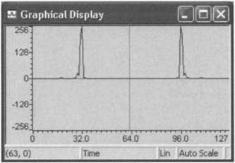
After properly configuring the PIP and SWI objects, the program is built. The entire DSP/BIOS version of the FFT files are provided on the accpompanying CD-ROM. In order to verify the operation of the DSP/BIOS-based FFT program, connect a function generator to the DSK board and run the program. Figure 10-34 shows a snapshot of the CCS animation feature. This is done by setting a breakpoint at the end of the FFT function and by opening a graphical display window via the menu item View → Graph → Time/Frequency. Place the global variable mag in the field Start Address to display the FFT magnitude values. Then, select the menu item Debug → Animate to start the animation. As the input frequency from the function generator is changed, the peaks in the graphical display window should move accordingly.
The FFT magnitude can be sent to the PC host by using the DMA as discussed in Lab 6.
When using DSK, the host-target data transfer is achieved by RTDX via the JTAG interface. Since the magnitude of the FFT is always stored into the variable mag, there is no need to deploy circular buffering as done in Lab 6. To configure RTDX, a RTDX object for output, ochan, is inserted at Input/Output category of the DSP/BIOS configuration. After the initialization via the RTDX_enableOutput ( ) API, the RTDX_write ( ) API is used to write a new mag to the output channel.
As shown next, the function HostTargetComm ( ) can be used to perform the same operation when using EVM:
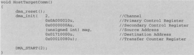
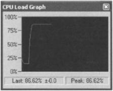
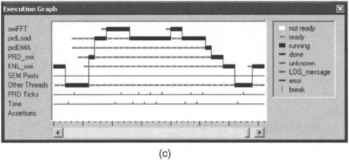
The DMA uses the global variable mag as the source address and the memory location 0x0171000, which is dedicated for FIFO access in PCI bus transfers, as the destination address. The program Host.exe, provided on the accompanying CD-ROM, is written to display the FFT magnitude on the PC monitor. This program makes use of the EVM API evm6x_read ( ). This API transfers data from the DSP to the host. In this lab, a PRD object prdComm is created and configured to run the host-target communication function HostTargetComm ( ) every 8 msec, as shown in Figure 10-35. After adding the HostTargetComm ( ) function to the FFT program, build the program and run it. To observe the FFT magnitude in real-time, also run Host.exe. The CPU load Graph plug-in can be used to verify that the DMA transfers the contents of mag independently of the CPU. As shown in Figure 10-36, the CPU load remains almost the same while the DMA transfer is running. To invoke the CPU load Graph plug-in, choose the menu item DSP/BIOS → CPU Load Graph.
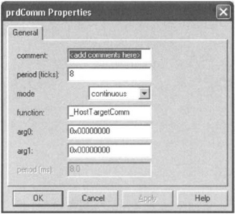
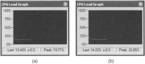
Figure 10-36 CPU Load Graph; (a) CPU load before DMA transfer, b) CPU load while DMA transfer is running.
L8.1 Prioritization of Threads
Instead of using the function generator to generate input samples, a CD player can be connected to the input jack of the audio daughter card. Of course, a pair of amplified speakers should be connected to the output jack of the daughter card to hear the sound. Now, let us examine the effect on the sound quality by changing the CPU load. To change the CPU load, a PRD object prdLoad is created and configured to run the function change load ( ) every 8 msec, as illustrated in Figure 10-37. The function changeload ( ) calls the otherProcessing ( ) function. The CPU load is determined by the global variable loadVal, which is passed to the otherProcessing ( ) function. The function changeload ( ) is shown next:
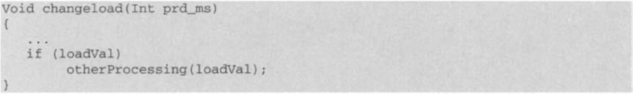
The global variable loadVal can be set by choosing Edit → Edit Variable to invoke the Edit Variable dialog box. In this dialog box, write loadVal in the field variable and the desired number in the field value. The prdLoad object will run the changeload ( ) function every 8 msec.
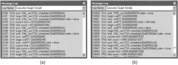
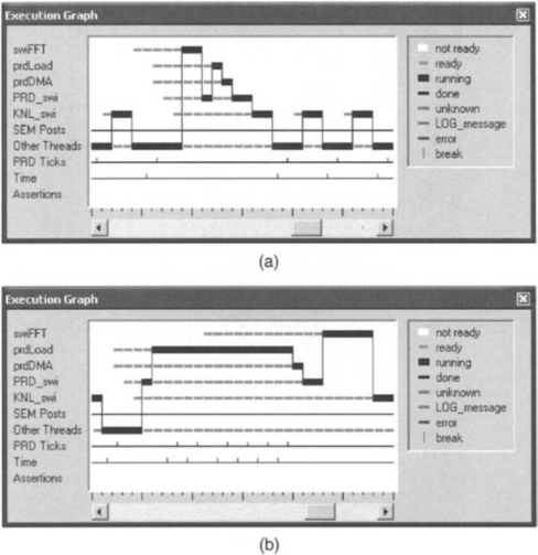
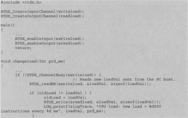
To observe the impact of the CPU load, let us build the program and run it while playing a CD. When the loadVal is changed to 900, the CPU load increases to about 87%, as shown in Figure 10-37, and the sound quality is degraded. The reason for this degradation can be seen by activating the Execution Graph Details window. As shown in Figure 10-38(a), when loadVal is zero, the swiFFT and PRD_swi threads complete their tasks without any problem. However, when loadVal is 900, these threads cannot complete their tasks and frequently go into the ready state, as shown in Figure 10-38(b). The Execution Graph in Figure 10-39 provides a graphical display of this situation. Since the swiFFT thread is competing with the PRD_swi thread, for large load values, the fft ( ) function sits waiting to be executed. The PRD_swi thread executes all the PRD objects, so it eventually runs the CPU load function otherProcessing ( ). Consequently, since the audio from the CD player is copied into the output frame by the fft ( ) function as part of the swiFFT thread, the sound quality suffers.
To solve this problem, the threads need to be properly prioritized. Let us assign a higher priority to the swiFFT thread. One simple way to do this is via the drag-and-drop method. Click on SWI – Software Interrupt Manager under Scheduling category in the Configuration Tool. On the right side of the window, click and hold the left mouse button on the PRD_swi icon, drag it to Priority 1, and release the button to drop it. This way the priority of the PRD_swi thread becomes 1. Similarly, move the swiFFT icon to Priority 2 so that it gets a higher priority than PRD_swi. Now build the program and run it. The sound quality remains unaffected even though loadVal = 900. The DSP/BIOS plug-ins in Figure 10-40 illustrate that the swiFFT thread no longer waits to be executed. Notice that the CPU load is now about 87%.
L8.2 RTDX
The CPU load can be changed by using the RTDX module. This module allows loadVal to be transferred from the host to the DSP while the program is running. The following piece of code shows the parts to be added to the original program to access the RTDX module (the entire program is provided on the accompanying CD):
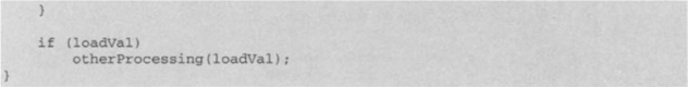
In order to use the indicated RTDX APIs, the program should include the header file rtdx.h. The RTDX input channel structure is declared and initialized by the macro RTDX_CreateInputChannel. Since it is declared as a global variable, it can be accessed anywhere in the program. Similarly, the RTDX_CreateOutputChannel macro defines and initializes the RTDX output channel structure. Because these channels are disabled during the initialization, they need to be enabled in main ( ) by using the RTDX_enableInput ( ) and RTDX_enableOutput ( ) APIs. The input channel is examined by the RTDX_channelBusy ( ) API to see whether it is busy or not. If it is not busy, data is read from the input channel by using the RTDX_readNB ( ) API. This API posts a request to the RTDX host library that the DSP application program is ready to receive data. The DSP program keeps running at this point. When the RTDX_read ( ) API is used, the DSP program stops until it receives data from the input channel. The RTDX_write ( ) API is used to write a new loadVal to the output channel in order to notify the host that such a value is received and used.
On the PC host side, an OLE application is written in Visual Basic to receive and send data. Build the program and run it. Then, run the OLE application embedded in rtdx.doc (provided on the accompanying CD-ROM). The CCS should be running when using RTDX. In addition the readload and writeload channels must be enabled by toggling the checkbox from the menu Tools → RTDX → Channel Viewer Control. It can be observed that the CPU load changes as a new loadVal is sent from the host OLE program to the DSP.