16

Kernel Tuning and Managing Performance Profiles with tuned

As described occasionally in previous chapters, each system performance profile must be adapted to the expected usage of our system.

Kernel tuning plays a key role in this optimization, and in this chapter, we will be exploring this further in the following sections:

• Identifying processes, checking memory usage, and killing processes
• Adjusting kernel scheduling parameters to better manage processes
• Installing tuned and managing tuning profiles
• Creating a custom tuned profile
• Using the web console for observing performance metrics

By the end of this chapter, you will understand how kernel tuning is applied, how quick profiles can be used via tuned to suit general use cases for different system roles, and how to further extend those customizations for your servers.

Additionally, identifying processes that have become a resource hog and how to terminate them and/or prioritize them will be a useful way of getting a bit more juice out of our hardware when most needed.

Let’s get hands-on and learn about these topics!

Technical requirements

You can continue the practice of using the virtual machine (VM) created at the beginning of this book in Chapter 1, Getting RHEL Up and Running. Any additional packages required for this chapter will be indicated alongside the text.

Identifying processes, checking memory usage, and killing processes

A process is a program that runs on our system—it might be a user logged in via Secure Shell (SSH) that has a bash terminal process running, or even the portion of the SSH daemon listening and replying to remote connections. Alternatively, it could be a program such as a mail client, a file manager, or more being executed.

Of course, processes take up resources in our system: memory, Central Processing Unit (CPU), disk, and more. Identifying or locating ones that might be misbehaving is a key task for system administrators.

Some of the basics were already covered in Chapter 4, Tools for Regular Operations, but it would be a good idea to have a refresher on these before continuing. However, here, we will be showing and using some of those tools in the context of performance tuning, such as the top command, which allows us to see processes and sort lists based on CPU usage, memory usage, and more. (Check the output of man top for a refresher on how to change the sorting criteria.)

One parameter to watch while checking system performance is the load average, which is a moving average made by the processes that are ready to run or are waiting for input/output (I/O) to complete. It’s composed of three values—1, 5, and 15 minutes—and gives an idea of whether a load is increasing or decreasing. A rule of thumb is that if a load average is below 1, there is no resource saturation.

The load average is shown alongside many other tools, such as the aforementioned top , uptime or w commands.

If the system-load average is growing, the CPU or memory usage is spiking, and if some processes are listed there, they will be easier to locate in the top output. If the load average is also high and increasing, it might be possible that the I/O operations are increasing it. It is possible to install the iotop package, which provides the iotop command to monitor disk activity. When executed, it will show the processes in the system and the disk activity related to each one—that is, reads, writes, and swaps that might give us some more hints about where to look.

Once a process has been identified as taking too many resources, we can send a signal to control it.

A signal list can be obtained with the kill –l command, as illustrated in the following screenshot:

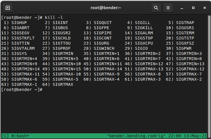
Figure 16.1 – Available signals to send to the processes

Note that each signal contains a number and a name—both can be used to send the signal to the process via its process identifier (PID).

Let’s review the most common ones, as follows:

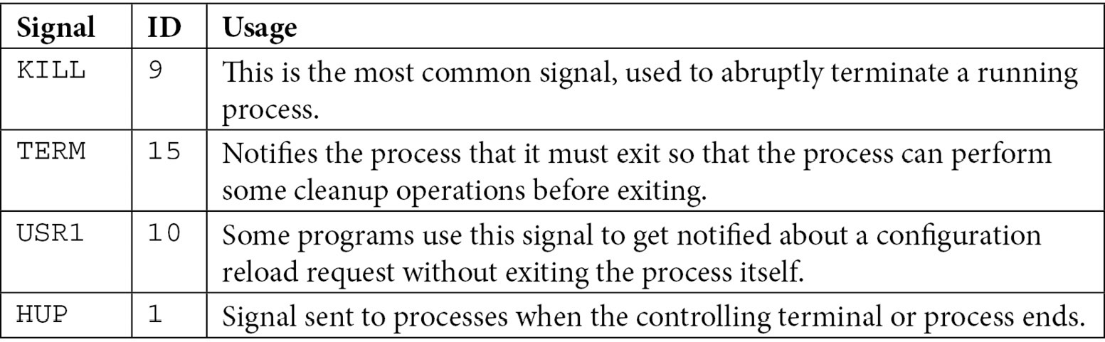
Table 16.1 – Signal names, IDs, and their common usage

From the list shown in Figure 16.1, it’s important to know that each signal has a disposition—that is, once a signal is sent, the process must, according to the signal received, perform one of the following actions: terminate, ignore the signal, perform a core dump, stop the process, or continue the process if it was stopped. The exact details about each signal can be checked at man 7 signal, as illustrated in the following screenshot:

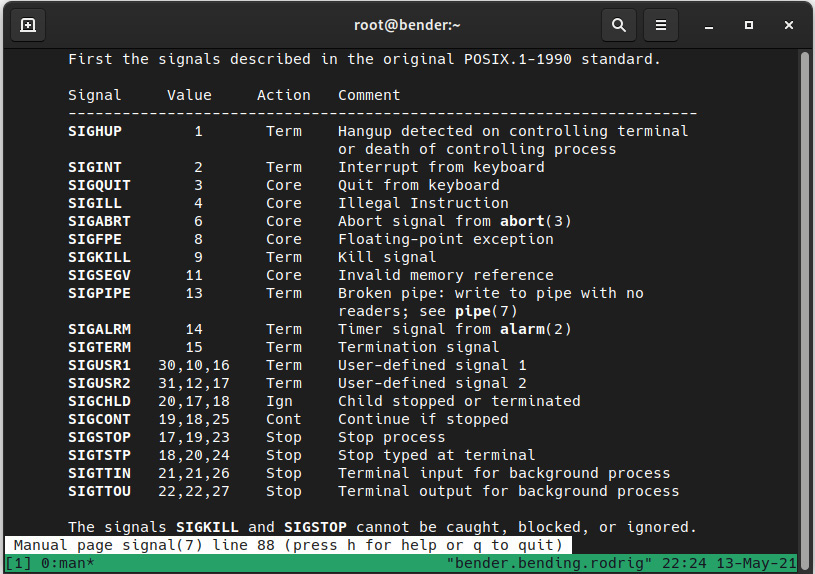
Figure 16.2 – The listing of signals, number equivalents, disposition (action), and behavior (man 7 signal)

One of the most typical usages when arriving at this point is to terminate processes that are misbehaving, so a combination of locating the process, obtaining the PID, and sending a signal to it is a very common task. In fact, it is so common that there are even tools that allow you to combine these stages in one command.

For example, we can compare ps aux|grep -i chrome|grep –v grep|awk '{print $2}'|xargs kill –9 with pkill –9 –f chrome. Both will perform the same action: search for processes named chrome, and send signal 9 (kill) to them.

Of course, even a user logging in is a process in the system (running SSH or the login shell, and so on); we can find the processes started by our target user via a similar construction (with ps, grep, and more) or with pgrep options such as pgrep –l –u user.

Bear in mind that, as the signals indicate, it’s better to send a TERM signal to allow the process to run its internal cleanup steps before exiting, as directly killing them might result in leftovers in our system.

One interesting command that was widely used before terminal multiplexers such as tmux or screen became commonplace was nohup, which was prepended to commands that would last longer—for example, downloading a big file. This command captured the terminal hangout signal, allowing the executed process to continue execution, storing the output in a nohup.out file that could be checked later.

For example, to download the latest Red Hat Enterprise Linux (RHEL) Image Standard Optical (ISO) file from the customer portal, select one release—for example, 9.0. Then, once logged in at https://access.redhat.com/downloads/content/479/ver=/rhel---9/9.0/x86_64/product-software, we will select the binary ISO and right-click to copy the Uniform Resource Locator (URL) for the download.

Tip

The URLs obtained when copying from the customer portal are timebound, meaning they are only valid for a short period of time. Afterward, the download link is no longer valid and a new one should be obtained after refreshing the URL.

In a terminal, we will then execute the following command with the copied URL:

nohup wget URL_OBTAINED_FROM_CUSTOMER_PORTAL &

With the preceding command, nohup will not close the processes on terminal hang-up (disconnection), so wget will continue downloading the URL. The end ampersand symbol (&) detaches the execution from the active terminal, leaving it as a background job that we can check with the jobs command until it has finished.

If we forget to add the ampersand, the program will block our input, but we can press Ctrl + Z on the keyboard to stop the process. However, since we really want it to be continuing execution but in the background, we will execute bg, which will continue the execution of it.

If we want to bring back the program to receive our input and interact with it, we can move it to the foreground using the fg command.

If we press Ctrl + C instead, while the program has our input, it will receive a petition to interrupt and stop execution.

You can see that workflow in the following screenshot:

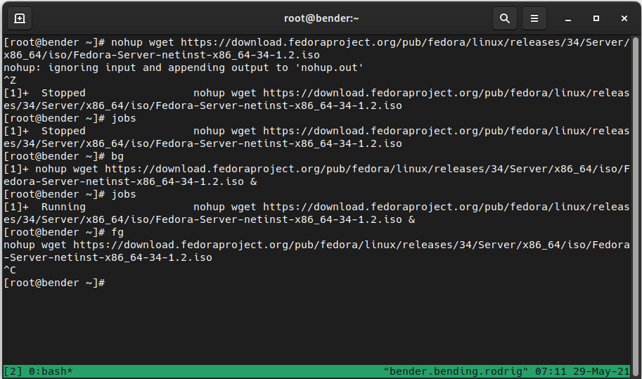
Figure 16.3 – Suspending the process, resuming to the background, bringing it to the foreground, and aborting

In this case, we’re downloading the Fedora 34 installation ISO (8 gigabytes or GB) using nohup and wget. Because we forgot to add the ampersand, we executed Ctrl + Z (which appears on the screen as ^Z).

The job was reported as job [1] with a status of Stopped (which is also reported when executing jobs).

Then, we bring the job to the background execution with bg, and now jobs reports it as Running.

Afterward, we bring the job back to the foreground with fg and execute Ctrl + C, represented as ^C on the screen, to finalize it.

This feature enables us to run multiple background commands—for example, we can copy a file in parallel to several hosts, as illustrated in the following screenshot:

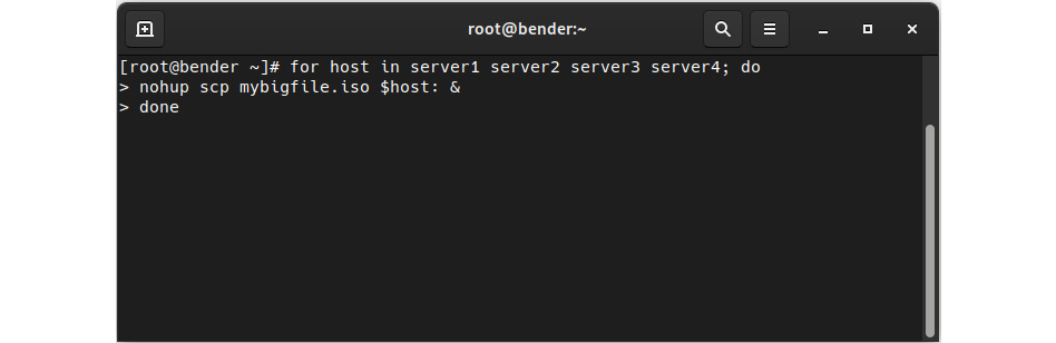
Figure 16.4 – Sample for the loop to copy a file to several servers with nohup

In this example, the copy operation performed over scp will be happening in parallel, and in the event of a disconnection from our terminal, the job will continue the execution and the output will be stored in nohup.out files in the folder that we were executing from.

Important Note

Processes launched with nohup will not be getting any additional input, so if the program asks for input, it will just stop execution. If the program asks for input, it’s recommended that you use tmux instead, as it will still protect from terminal disconnection but also allow interaction with the launched program.

We will not always be willing to kill processes or stop or resume them; we might just want to deprioritize or prioritize them—for example, for long-running tasks that might not be critical.

Let’s learn about this feature in the next section.

Adjusting kernel scheduling parameters to better manage processes

The Linux kernel is a highly configurable piece of software, so there’s a whole world of tunables that can be used for adjusting its behavior: for processes, network cards, disk, memory, and more.

The most common tunables are the nice process value and the I/O priority, which regulate, respectively, the prioritization versus other processes of the CPU and I/O time.

For interacting with processes we’re about to start, we can use the nice or ionice commands, prepending the command we want to execute with some parameters (remember to check the man contents for each one to get the full available range of options). Just remember that for nice, processes can go from –20 to +19, with 0 being the standard one, -20 the highest priority, and 19 the lowest priority (the higher the value, the nicer the process is).

Each process has a likelihood of getting kernel attention to run. By changing the priority via nice before execution or via renice once it’s running, we can alter it a bit.

Let’s think about a long-running process such as performing a backup—we want the task to succeed, so we will not be stopping or killing the process. However, at the same time, we don’t want it to alter the production or level of service of our server. If we define the process with a nice value of 19, this means that any process in the system will get more priority—that is, our process will keep running but will not make our system busier.

This gets us into an interesting topic—many new users arriving in the Linux world, or administrators of other platforms, get a shock when they see that the system, with plenty of memory (random-access memory or RAM), is using swap space or that the system load is high. It is clear that some slight usage of swap space and having lots of free RAM just means that the kernel has optimized the usage by swapping out unused memory to disk. As long as the system doesn’t feel sluggish, having a high load just means that the system has a long queue of processes to be executed; however, if the processes are niced to 19, for example, they are in the queue, as mentioned, any other process will go ahead of it in terms of priority.

When we’re checking the system status with top or ps, we can also check for how long a process has been running, and that is also accounted for by the kernel. A new process just created that starts eating CPU and RAM has a higher chance of being killed by the kernel to ensure system operability (remember the out-of-memory (OOM) killer mentioned in Chapter 4, Tools for Regular Operations?).

For example, let's use renice on the process running our backup (containing the backup pattern in the process name to the lowest priority) with the following code:

pgrep –f backup | xargs renice –n 19

143405 (process ID) old priority 0, new priority 19

144389 (process ID) old priority 0, new priority 19

2924457 (process ID) old priority 0, new priority 19

3228039 (process ID) old priority 0, new priority 19

As you can see, pgrep has collected a list of PIDs, and that list has been piped as arguments for renice with a priority adjustment of 19, making processes nicer to others actually running in the system by giving others more chances to use CPU time.

Let’s repeat the preceding example in our system by running a pi (π) calculation using bc, as illustrated in the man page for bc. First, we will time how long it takes for your system. Then, we will execute it via renice. So, let’s get hands-on—first, let’s time it, as follows:

time echo "scale=10000; 4*a(1)" | bc –l # Letter lowercase L

In my system, this was the result:

3.141592653...

...

375676

real 3m8,336s

user 3m6,875s

sys  0m0,032s

Now, let’s run it with renice, as follows:

time echo "scale=10000; 4*a(1)" | bc -l &

pgrep –f bc |xargs renice –n 19 ; fg

In my system again, this was the result:

real 3m9,013s

user 3m7,273s

sys  0m0,043s

There’s a slight difference of 1 second, but you can try running more processes to generate system activity in your environment to make it more visible and add more zeros to the scale to increase the time of execution. Similarly, ionice can adjust the priority of I/O operations that a process is causing (reads and writes)—for example, by repeating the action over the processes that take care of creating our backups, we could run the following command:

pgrep –f  backup|xargs ionice –c 3 –p

By default, it will not output information, but we can check the value via execution of the following command:

pgrep -f backup|xargs ionice -p

idle

idle

idle

idle

In this case, we’ve moved our backup processes so that I/O requests are handled when the system is idle.

The class, which we specified with the –c argument, can be one of the following:

• 0: None
• 1: Real-time
• 2: Best-effort
• 3: Idle

With –p, we specify the processes to act on.

Most of the settings that we can apply to our system came from specific ones, applied to each PID via the /proc/ virtual filesystem, such as adjusting the oom_adj file to reduce the value shown in the oom_score file. In the end, this determines whether the process should be higher on the list when OOM has to kill some process to try saving the system from catastrophe.

Of course, there are system-level settings such as /proc/sys/vm/panic_on_oom that can tune how the system has to react (panic or not) if OOM has to be invoked.

Additionally, the disks have a setting to define the scheduler being used—for example, for a disk named sda, it can be checked via cat /sys/block/sda/queue/scheduler.

The scheduler used for a disk has different approaches and depends on the kernel version—for example, in RHEL 7, it used to be noop, deadline, or cfq. However, in RHEL 8 and RHEL 9, those were removed, so we have md-deadline, bfq, kyber, and none.

This is such a big and complex topic that there is even a specific manual for it at https://access.redhat.com/documentation/en-us/red_hat_enterprise_linux/9/html-single/monitoring_and_managing_system_status_and_performance/index. So if you’re interested in going deeper, have a look at it.

I hope to have achieved two things here, as follows:

• Making clear that the system has a lot of options for tuning and that it has its own documentation for it, even a Red Hat Certified Architect exam at https://www.redhat.com/en/services/training/rh442-red-hat-enterprise-performance-tuning.
• It’s not an easy task—one idea has been reinforced several times in this book: test everything using your system’s workload, as results might vary from one system to another.

Fortunately, there’s no need to feel afraid about system tuning—it’s something we can become more proficient in with experience at all levels (including knowledge, hardware, workloads, and more). But on the other hand, systems also include some easier ways to perform quick adjustments that will fit many scenarios, as we will see in the next section.

Installing tuned and managing tuning profiles

Hopefully, after a bit of scaremongering happening in the previous section, you already have a mindset prepared for an easier path.

Just in case, ensure the tuned package is installed, or install it with dnf –y install tuned. The package provides a tuned service that must be enabled and started for operation. As a refresher, we can achieve this by running the following command:

systemctl enable tuned

systemctl start tuned

Now we’re ready to interact and get more information about this service, which announces itself at dnf info tuned as a daemon that tunes the system dynamically based on observation and is currently acting on an Ethernet network and hard disks.

Interaction with the daemon is performed via the tuned-adm command. For illustration, in the following screenshot, we’re showing the command-line options that are available and a list of profiles:

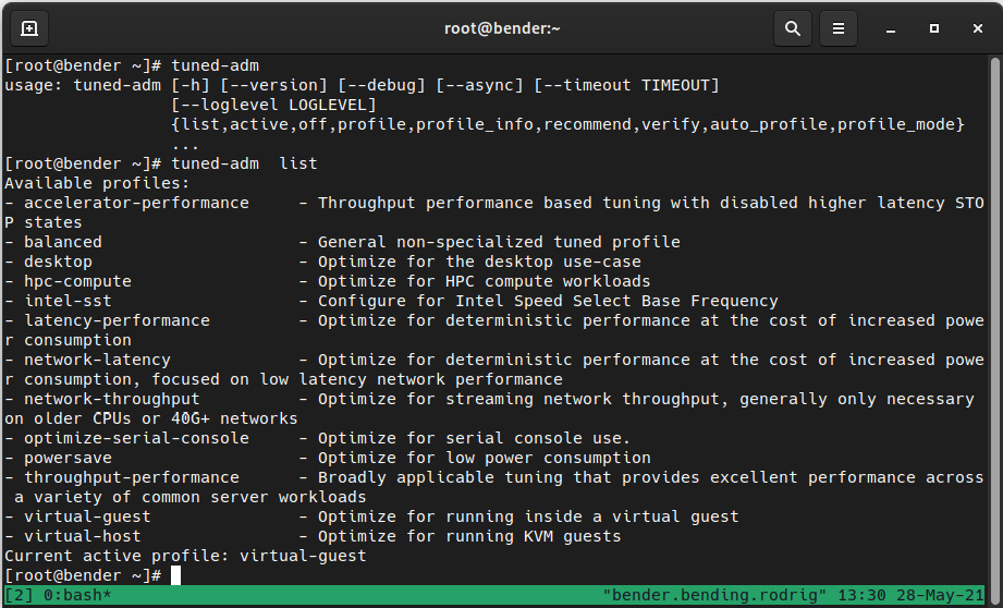
Figure 16.5 – The tuned-adm command-line options and profiles

As you can see, there are some options for listing, disabling, and grabbing information about a profile, getting recommendations about which profile to use, verifying that settings have not been altered, automatically selecting a profile, and more.

One thing to bear in mind is that newer versions of the tuned package might bring additional profiles or configurations (stored in the /usr/lib/tuned/ folder hierarchy), so the output might differ in your system.

Let’s review some of the most common ones in the following table:

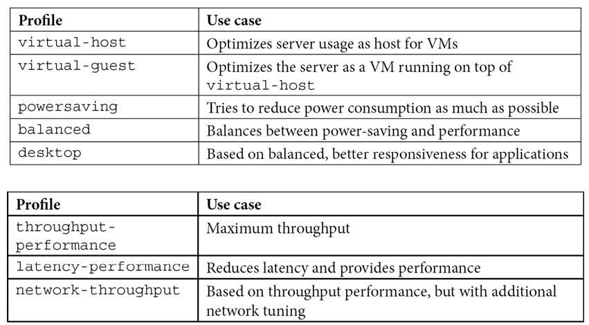
Table 16.2 – The tuned-adm profiles and use cases

As mentioned earlier, each configuration is always a trade-off—more power consumption is required when increasing performance; otherwise, improving throughput might also increase latency.

Let’s enable the latency-performance profile for our system. To do so, we will execute the following command:

tuned-adm profile latency-performance

We can verify that it has been activated with tuned-adm active, where we can see it shows latency-performance, as shown in the following screenshot:

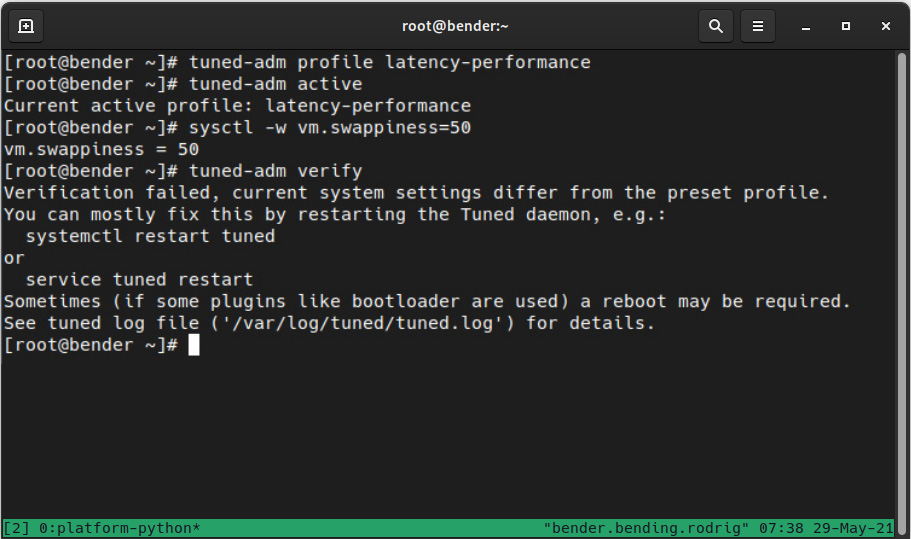
Figure 16.6 – The tuned-adm profile activation and verification

Additionally, we modified the system with sysctl -w vm.swappiness=69 (on purpose) to demonstrate the tuned-adm verify operation, as it reported that some settings changed from the ones defined in the profile.

Important Note

As of writing, dynamic tuning is disabled by default—to enable or to check the current status, check that dynamic_tuning=1 appears in the /etc/tuned/tuned-main.conf file. It is disabled in the performance profiles as, by default, it tries to balance power consumption and system performance, which is the opposite of what performance profiles try to do.

Additionally, bear in mind that the Cockpit interface introduced in this book also features a way to change the performance profile, as shown in the following screenshot. Once you have clicked on the Performance profile link from the main Cockpit page, you will see this dialog open:

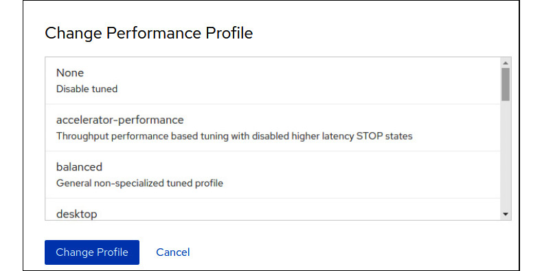
Figure 16.7 – Changing the tuned profile within the Cockpit web interface

In the next section, we will examine how tuned profiles work under the hood and how to create a custom one.

Creating a custom tuned profile

Once we’ve commented on the different tuned profiles, we can ask the following questions: How do they work? How do we create one?

For example, let’s examine latency-performance in the next lines of code, by checking the /usr/lib/tuned/latency-performance/tuned.conf file.

In general, the syntax of the file is described in the man tuned.conf page, but the file, as you will be able to examine, is an initialization (ini) file—that is, a file organized in categories, expressed between brackets and pairs of keys and values assigned by the equals (=) sign.

The main section defines a summary of the profile if it inherits from another profile via include, and the additional sections depend on the plugins installed.

To learn about the available plugins, the documentation included on the man page (man tuned.conf) instructs us to execute rpm -ql tuned | grep 'plugins/plugin_.*.py$', which provides an output similar to this:

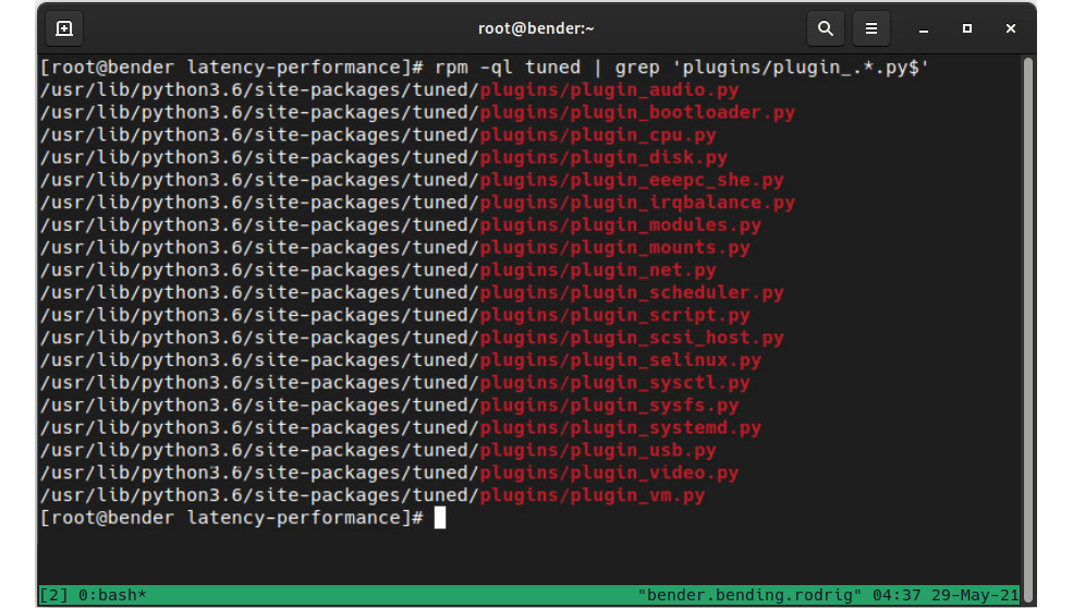
Figure 16.8 – The available tuned plugins in our system

Important Note

If two or more plugins try to act over the same devices, the replace=1 setting will mark the difference between running all of them or only the latest one.

Coming back to the latency-performance profile, this has three sections: main, cpu, and sysctl.

For the CPU, it sets the performance governor, which we can check—if supported via cat /sys/devices/system/cpu/*/cpufreq/scaling_governor—for each CPU that is available in our system. Bear in mind that in some systems, the path might differ or might not even exist, and we can check the available ones via the execution of cpupower frequency-info –governors, with powersave and performance being the most common ones.

The name of the section for each plugin might be arbitrary if we specify the type keyword to indicate which plugin to use, and we can use some devices to act on via the devices keyword, allowing—for example—the definition of several disk sections with different settings based on the disk being configured. For example, we might want some settings for the system disk—let’s say sda—that are different for the disk, so we use the data backups at sdb, as illustrated here:

[main_disk]
type=disk
devices=sda
readahead=>4096
[data_disk]
type=disk
devices=!sda
spindown=1

In the preceding example, the disk named sda gets configured with readahead (which reads sectors ahead of the current utilization to have the data cached before actually being requested to access it), and we’re telling the system to use spindown on data disks that might only be used at backup time, thus reducing noise and power consumption when not in use.

Another interesting plugin is sysctl, used by several of the profiles, which defines settings in the same way as the sysctl command. Because of this, the possibilities are huge: defining the Transmission Control Protocol (TCP) window sizes for tuning networking, virtual memory management, transparent huge pages, and more.

Tip

It is hard to start from scratch with any performance tuning, and as tuned allows us to inherit settings from a parent, it makes sense to find which one of the available profiles is the closest to what we want to achieve, check what is being configured in it, and—of course—compare it with the others (as you can see, there are also examples for other plugins) and apply it to our custom profile.

To get an idea about how the defined system profiles touch a system, my RHEL 9 system shows the following output for cat /usr/lib/tuned/*/tuned.conf|grep -v ^#|grep '^['|sort –u:

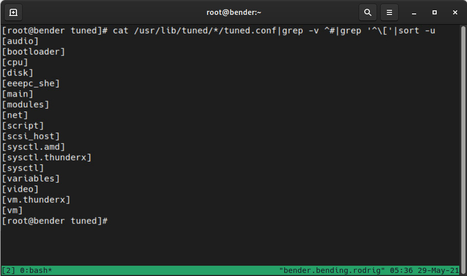
Figure 16.9 – Sections in the system-supplied profiles

So, as you can see, they touch a lot of areas. I would like to highlight the script section, which defines a shell script to execute used by the powersave profile, and the variables section, used by throughput-performance to define regular expressions for later matching and applying settings based on the CPU.

Once we’re ready, we will create a new folder at /etc/tuned/newprofile. A tuned.conf file must be created, containing the main section with the summary and additional sections for the plugins we want to use.

When creating a new profile, it might be easier if we copy the profile we’re interested in from the /usr/lib/tuned/$profilename/ into our /etc/tuned/newprofile/ folder and start the customization from there.

Once it’s ready, we can enable the profile with tuned-adm profile newprofile, as we introduced earlier in this chapter.

You can find more information about the profiles available in the official documentation at https://access.redhat.com/documentation/en-us/red_hat_enterprise_linux/9/html-single/monitoring_and_managing_system_status_and_performance/index#tuned-profiles-distributed-with-rhel_getting-started-with-tuned.

With this, we’ve set up our own custom profile for tuning our performance settings.

In the next section, let’s explore how to graphically check the performance of our system.

Using the web console for observing performance metrics

Having adjusted the tuned profile or even having a custom one defined, as we covered earlier in this chapter, requires a confirmation that our changes are there and improving the performance... and a very good fit for this is using the web console for obtaining this data.

Just in case, make sure that you enable the cockpit service by executing systemctl enable --now cockpit.socket. Once enabled, you can connect the IP address of the host at port 9090 with your browser to get access to it.

In my case, the IP of the host is 192.168.2.60 and the final URL is https://192.168.2.60:9090, which, when accessed, shows this warning in the browser:

Figure 16.10 – Security warning when accessing a non-trusted certificate

When clicking on Advanced, we get the following dialog:

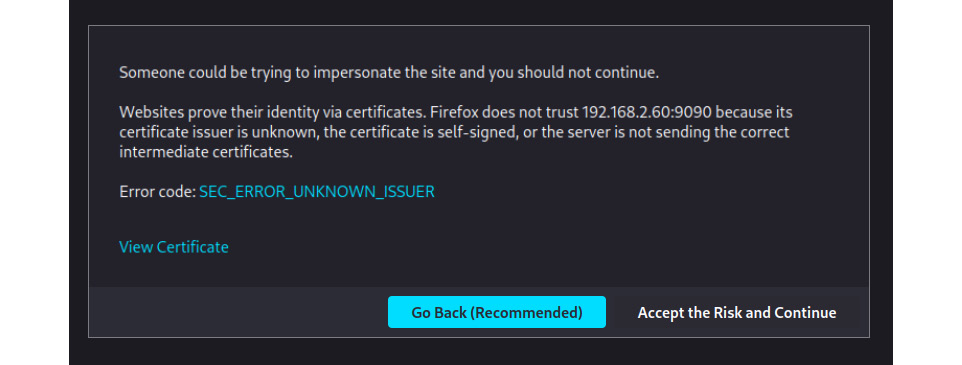
Figure 16.11 – The advanced non-trusted SSL certificate dialog in the browser

Let’s click on Accept the Risk and Continue so that we get to the login screen of Cockpit:

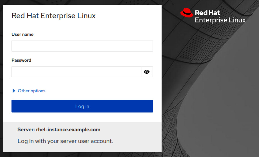
Figure 16.12 – The Cockpit login screen

After entering your user credentials (in my case, I used the root user), we get to the dashboard screen, as follows:

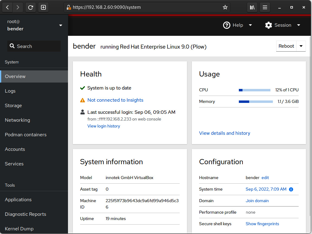
Figure 16.13 – The Cockpit dashboard after login

When we click on the View details and history option under Usage, we get to the following screen:

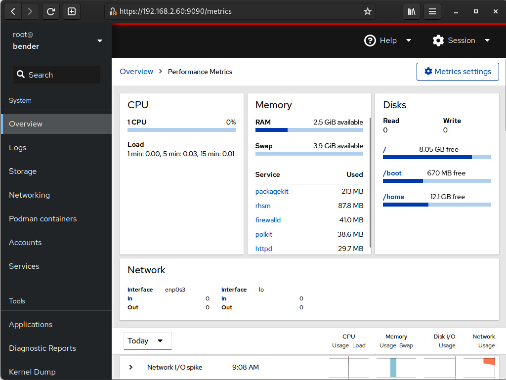
Figure 16.14 – The Cockpit usage information requesting additional packages for historical data

As we can see, Cockpit informs us that we’re missing the cockpit-pcp package for grabbing metrics history:

Figure 16.15 – Additional software installation dialog in Cockpit

Bear in mind that if the package was missing, once enabled, it will take a while to start reporting metrics and events. But once this has been done, you can see a new section similar to this one:

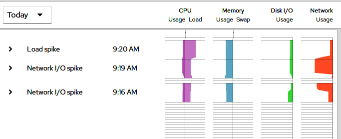
Figure 16.16 – Cockpit performance information once pmlogger has been running for a while in our system

As you can see, we can quickly evaluate the data obtained and the events recorded to match against known bottlenecks with our system. Using this data, we can check whether the performed changes in the tuned profiles of other settings have improved the overall system experience.

Note that Cockpit uses Performance Copilot (pcp) in the background for collecting information about our system and showing it graphically. Remember that this is only a graphical interface and that other tools might be available in our system for this task.

With these guidelines, we come to the end of this chapter.

Summary

In this chapter, we learned about identifying processes, checking their resource consumption, and how to send signals to them.

In terms of the signals, we learned that some of them have some additional behavior, such as terminating processes nicely or abruptly, simply sending a notification that some programs understand as reload configuration without restarting, and more.

Also, related to processes, we learned how to adjust their priority compared to other processes in terms of CPU and I/O so that we can adjust long-running processes or disk-intensive ones to not affect other running services.

Finally, we introduced the tuned daemon, which includes several general use-case profiles that we can use directly in our system, allowing tuned to apply some dynamic tuning. Alternatively, we can fine-tune the profiles by creating one of our own to increase system performance or optimize power usage. We also learned how to graphically monitor the performance of our system via the cockpit web console that provides additional tools and allows us to evaluate the outcome of the tunings performed.

In the next chapter, we will learn about how to work with containers, registries, and other components so that applications can run as provided by the vendor while being isolated from the server running them.