4

Tools for Regular Operations

At this point in this book, we’ve installed a system, and we’ve covered some of the scripts we can create to automate tasks, so we’ve reached the point where we can focus on the system itself.

Having a system properly configured requires not only installing it but understanding how to run tasks at specific times, keeping all the services running appropriately, and configuring time synchronization, service management, boot targets (runlevels), and scheduled tasks, all of which we will be covering in this chapter. We’ll be additionally starting to mention Cockpit (web console), which will be covered during the whole book as a tool to perform administration tasks from a web interface.

In this chapter, you will learn how to check the statuses of services and how to start, stop, and troubleshoot them, as well as how to keep the system clock in sync for your server or your whole network.

The list of topics that will be covered is presented here:

• Managing system services with systemd
• Scheduling tasks with cron and systemd
• Learning about time synchronization with chrony and the Network Time Protocol (NTP)
• Checking for free resources—memory and disk (free and df)
• Finding logs, using journald, and reading log files, including log preservation and rotation

Technical requirements

It is possible for you to complete this chapter by using the virtual machine (VM) we created at the beginning of this book. Additionally, for testing the NTP server, it might be useful to create a second VM that will connect to the first one as a client, following the same procedure we used for the first one. Additionally, required packages will be indicated within the text.

Managing system services with systemd

In this section, you will learn how to manage system services, runtime targets, and all about the service status with systemd. You will also learn how to manage system boot targets and services that should start at system boot.

systemd (which you can learn a bit about at https://www.freedesktop.org/wiki/Software/systemd/) is defined as a system daemon that’s used to manage the system. It came as a rework of how a system boots and starts, and it looks at the limitations related to the traditional way of doing it.

When we think about the system starting, we have the initial kernel and ramdisk load and execution, but right after that, services and scripts take control to make filesystems available. This helps prepare the services that provide the functionality we want from our system, such as the following:

• Hardware detection
• Additional filesystem activation
• Network initialization (wired, wireless, and so on)
• Network services (time sync, remote login, printers, network filesystems, and so on)
• User-space setup

However, most of the tools that existed before systemd came into play worked on this in a sequential way, causing the whole boot process (from boot to user login) to become lengthy and be subject to delays.

Traditionally, this also meant we had to wait for the required service to be fully available before the next one that depended on it could be started, increasing the total boot time.

Some approaches were attempted, such as using Monit or other tools that allow us to define dependencies, monitor processes, and even recover from failures, but in general, it was reusing an existing tool to perform other functions, trying to win the race regarding the fastest-booting system.

Important Note

systemd redesigned the process to focus on simplicity: start fewer processes and do more parallel execution. The idea itself sounds easy but requires redesigning a lot of what was taken for granted in the past, to focus on the needs of a new approach to improve operating system performance.

This redesign, which has provided a lot of benefits, also came with a cost: it drastically changed the way systems booted, so there has been a lot of controversy on the adoption of systemd by different vendors, and even some efforts by the community to provide systemd-free variants.

Rationalizing how services start so that only those that are required are started is a good way to accomplish efficiency—for example, there is no need to start Bluetooth, printer, or network services when the system is disconnected, there is no Bluetooth hardware, or no one is printing. With fewer services waiting to start, the system boot is not delayed by those waits and focuses on the ones that really need attention.

On top of that, parallel execution allows us to have each service taking the time it needs to get ready but not make others wait, so in general, running services initialization in parallel allows us to maximize the usage of the central processing unit (CPU), disk, and so on, and the wait times for each service are used by other services that are active.

systemd also pre-creates listening sockets before the actual daemon is started, so services that have requirements on other services can be started and be on a wait status until their dependencies are started. This is done without them losing any messages that are sent to them, so when the service is finally started, it will act on all pending actions.

Let’s learn a bit more about systemd as it will be required for several operations we’re going to describe in this chapter.

systemd comes with the concept of units, which are nothing but configuration files. These units can be categorized as different types, based on their file extension, as illustrated in the following screenshot:

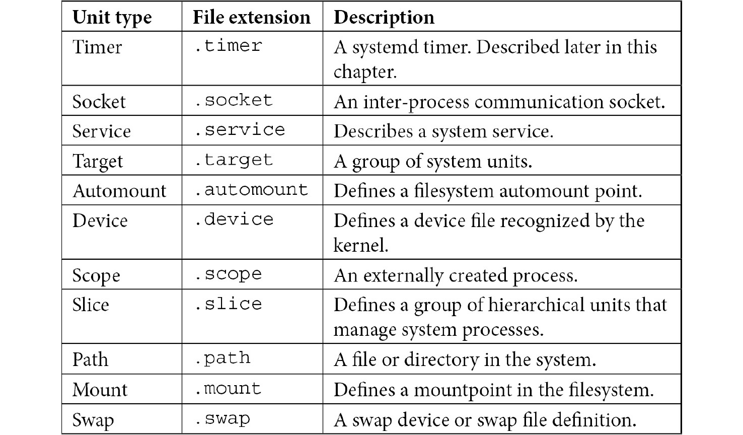
Table 4.1 – systemd unit types description

Tip

Don’t feel overwhelmed by the different systemd unit types. In general, the most common ones are service, timer, socket, and target.

Of course, these unit files are expected to be found in some specific folders, as shown here:

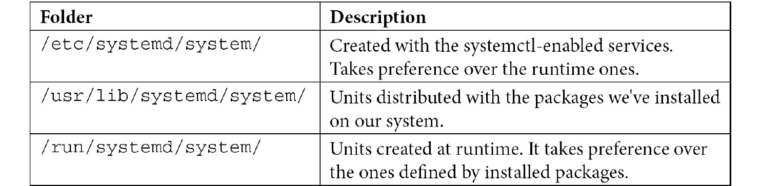
Table 4.2 – System folders containing systemd files

As we mentioned earlier about sockets, unit files for path, bus, and more are activated when a system’s access to that path is performed, allowing services to be started when another one is requiring them. This adds more optimization for lowering system startup times.

With that, we have learned about systemd unit types. Now, let’s focus on the file structure of unit files.

systemd unit file structure

Let’s get our hands dirty with an example: a system has been deployed with sshd enabled, and we need to get it running once the network has been initialized in the runlevels, which provide connectivity.

As we mentioned previously, systemd uses unit files, and we can check the aforementioned folders or list them with systemctl list-unit-files. Remember that each file is a configuration file that defines what systemd should do; for example, /usr/lib/systemd/system/chronyd.service, as shown in the following screenshot:

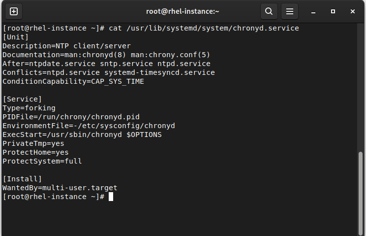
Figure 4.1 – chronyd.service contents

This file defines not only the traditional program to start and the process identifier (PID) file, but the dependencies, conflicts, and soft dependencies, which provides enough information to systemd to decide on the right approach.

If you’re familiar with INI files, this file uses that approach, in that it uses square brackets, [ and ], for sections and then pairs of key=value for the settings in each section.

Section names are case-sensitive, so they will not be interpreted correctly if the proper naming convention is not used.

Section directives are named like so:

• [Unit]
• [Install]

There are additional entries for each of the different types, as follows:

• [Service]
• [Socket]
• [Mount]
• [Automount]
• [Swap]
• [Path]
• [Timer]
• [Slice]

As you can see, we have specific sections for each type. If we execute man systemd.unit, it will give you examples, along with all the supported values, for the systemd version you’re using, as illustrated in the following screenshot:

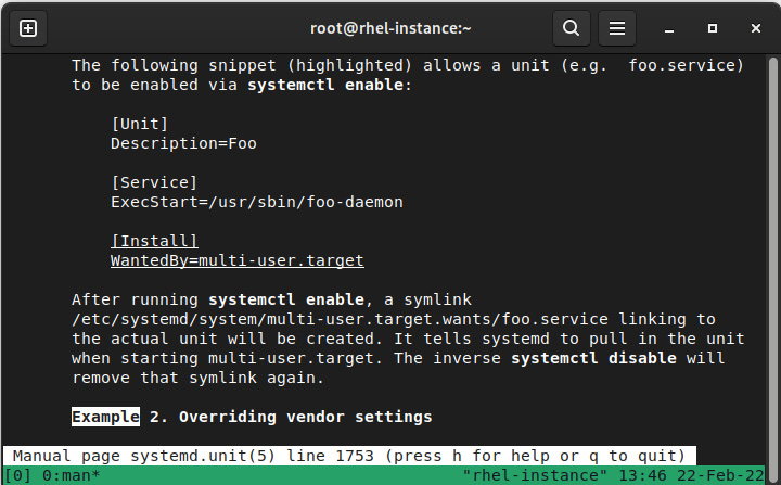
Figure 4.2 – Manual (man) page of systemd.unit

With that, we have reviewed the file structure of unit files. Now, let’s use systemctl to actually manage the service’s status.

Managing services to be started and stopped at boot

Services can be enabled or disabled; that is, the services will or won’t be activated on system startup.

If you’re familiar with the previous tools available in Red Hat Enterprise Linux (RHEL), it was common to use chkconfig to define the status of services based on their default rc.d/ settings.

The sshd service can be enabled via the following command:

#systemctl enable sshd

It can also be disabled via the following command:

#systemctl disable sshd

This results in creating or removing /etc/systemd/system/multi-user.target.wants/sshd.service. Notice multi-user.target in the path, which is the equivalent of the runlevel we used to configure other approaches such as initscripts.

Tip

Although traditional usage of chkconfig (once installed) is provided for compatibility so that chkconfig sshd on/off or service start/stop/status/restart sshd is valid, it is better to get used to the systemctl approach described in this chapter.

The previous commands enable or disable the service at boot, but for executing an immediate action, we need to issue different commands.

To start the sshd service, use the following command:

#systemctl start sshd

To stop it, use the following command:

#systemctl stop sshd

Of course, we can also check the service’s status. Here is an example of looking at systemd via systemctl status sshd:

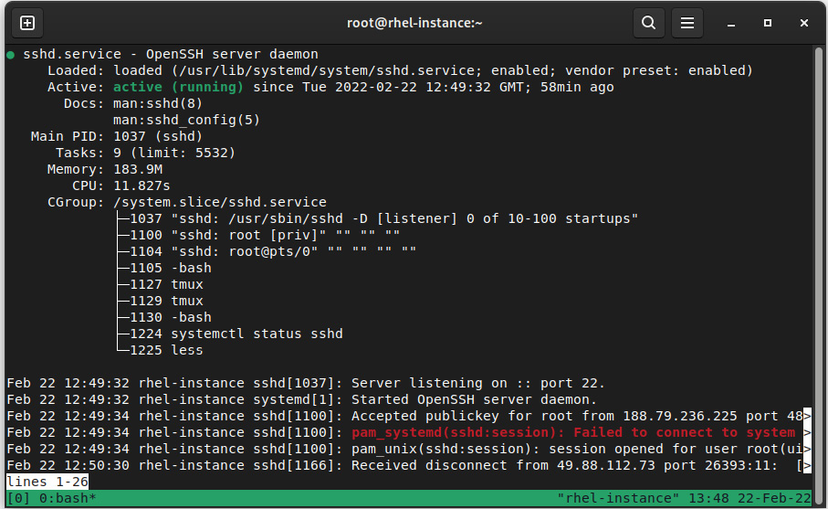
Figure 4.3 – Status of sshd daemon

This status information provides details about the unit file defining the service, its default status at boot, if it is running or not, its PID, some other details about its resource consumption, and some of the most recent log entries for the service, which are quite useful when you’re debugging simple service start failures.

One important thing to check is the output of systemctl list-unit-files as it reports the defined unit files in the system, as well as the current status and the vendor preset for each one.

Now that we have covered how to start/stop and status check services, let’s work on managing the actual system boot status itself.

Managing boot targets

The default status we have defined at boot is important when it comes to talking about runlevels.

A runlevel defines a predefined set of services based on usage; that is, they define which services will be started or stopped when we’re using a specific functionality.

For example, there are runlevels that are used to define the following:

• Halt mode
• Single-user mode
• Multi-user mode
• Networked multiuser
• Graphical UI
• Reboot

Each of those runlevels allows a predefined set of services to be started/stopped when the runlevel is changed with init $runlevel. Of course, levels used to be based on each other and were very simple, as outlined here:

• Halt stopped all the services and then halted or powered off the system.
• Single-user mode started a shell for one user.
• Multi-user mode enabled regular login daemons on the virtual terminals.
• Networked was like multi-user but with the network started.
• Graphical was like networked but with graphical login via display manager (gdm or others).
• Reboot was like halt, but at the end of processing services, it issued a reboot instead of a halt.

These runlevels (and the default one when the system is booted) used to be defined in /etc/inittab, but the file placeholder reminds us of the following:

# inittab is no longer used.
#
# ADDING CONFIGURATION HERE WILL HAVE NO EFFECT ON YOUR SYSTEM.
#
# Ctrl-Alt-Delete is handled by /usr/lib/systemd/system/ctrl-alt-del.target
#
# systemd uses 'targets' instead of runlevels. By default, there are two main targets:
#
# multi-user.target: analogous to runlevel 3
# graphical.target: analogous to runlevel 5
#
# To view current default target, run:
# systemctl get-default
#
# To set a default target, run:
# systemctl set-default TARGET.target

So, by making this change to systemd, a new way to check the available boot targets and define them is in place.

We can find the available system targets by listing this folder:

#ls -l /usr/lib/systemd/system/*.target

Or, more correctly, we can use systemctl, like so:

#systemctl list-unit-files *.target

When you examine the output on your system, you will find some compatibility aliases for runlevels 0 to 6 that provide compatibility with the traditional ones.

For example, for regular server usage, the default target will be multi-user.target when you’re running without graphical mode or graphical.target when you’re using it.

We can define, as instructed in the placeholder at /etc/inittab, the new runlevel to use by executing the following command:

#systemctl set-default TARGET.target

We can verify the active one by using the following command:

#systemctl get-default

This brings us to the next question: What does a target definition look like? Let’s examine the output in the following screenshot:

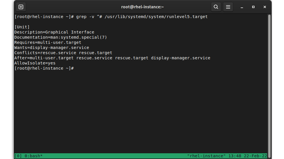
Figure 4.4 – Contents of runlevel 5 from its target unit definition

As you can see, it is set as a dependency of another target (multi-user.target) and has some requirements on other services, such as display-manager.service, and also other conflicts, and the target can only be reached when other targets have completed.

In this way, systemd can select the proper order of services to start and the dependencies to reach the configured boot target.

Just in case, we can switch to a new runlevel with systemctl isolate targetname.target.

With that, we have covered the service’s status, as well as how to start, stop, and enable it on boot, but there are other tasks we should execute in our system, but in a periodic way. Let’s get further into this topic.

Scheduling tasks with cron and systemd

The skills you will learn in this section will be concerned with scheduling periodic tasks in the system for business services and maintenance.

For regular system usage, there are tasks that need to be executed periodically, ranging from temporary folder cleanup, updating the cache’s refresh rate, and performing check-in with inventory systems, among other things.

The traditional way to set them up is via cron, which is provided in RHEL 9 via the cronie package.

cronie implements a daemon that’s compatible with the traditional Vixie cron and allows us to define both user and system crontabs.

A crontab defines several parameters for a task that must be executed. Let’s see how it works.

System-wide crontab

A system-wide crontab can be defined in /etc/crontab or in individual files at /etc/cron.d. Other additional folders exist, such as /etc/cron.hourly, /etc/cron.daily, /etc/cron.weekly, and /etc/cron.monthly.

In the folders for hourly, daily, weekly, or monthly, you can find scripts or symbolic links to them. When the period since the preceding execution is met (1 hour, 1 day, 1 week, 1 month), the script will be executed.

In contrast, in /etc/crontab or /etc/cron.d, as well as in the user crontabs, the standard definition of jobs is used.

Jobs are defined by specifying the parameters that are relevant to the execution period, the user that will be executing the job (except for user crontabs), and the command to execute, as illustrated in the following code snippet:

# Run the hourly jobs
SHELL=/bin/bash
PATH=/sbin:/bin:/usr/sbin:/usr/bin
MAILTO=root
01 * * * * root run-parts /etc/cron.hourly

By looking at the standard /etc/crontab file, we can check the meaning of each field, as follows:

# Example of job definition:
# .---------------- minute (0 - 59)
# |  .------------- hour (0 - 23)
# |  |  .---------- day of month (1 - 31)
# |  |  |  .------- month (1 - 12) OR jan,feb,mar,apr ...
# |  |  |  |  .---- day of week (0 - 6) (Sunday=0 or 7) OR sun,mon,tue,wed,thu,fri,sat
# |  |  |  |  |
# *  *  *  *  * user-name  command to be executed

Based on this, if we check the initial example, 01 * * * * root run-parts /etc/cron.hourly, we can deduce the following:

• Run at minute 01
• Run every hour
• Run every day
• Run every month
• Run every day of the week
• Run as root
• Execute the run-parts /etc/cron.hourly command

This, in brief, means that the job will run on the first minute of every hour as the root user and will run any script located in that folder.

Sometimes, it is possible to see an indication, such as */number, which means that the job will be executed every multiple of that number. For example, */3 will run every 3 minutes if it is on the first column, every 3 hours if it’s on the second, and so on.

Any command we might execute from the command line can be executed via cron, and the output will be—by default—mailed to the user running the job. It is a common practice to either define the user that will receive the email via the MAILTO variable in the crontab file or to redirect them to the appropriate log files for the standard output and standard error (stdout and stderr).

User crontab

As with the system-wide crontab, users can define their own crontabs so that tasks are executed by the user. This is, for example, useful for running periodic scripts both for a human user or a system account for a service.

The syntax for user crontabs is the same as it is system-wide. However, the column for the username is not there, since it is always executed as the user is defining the crontab itself.

A user can check their crontab via crontab –l, as follows:

[root@rhel-instance ~]# crontab -l

no crontab for root

A new one can be created by editing it via crontab -e, which will open a text editor so that a new entry can be created.

Let’s work with an example by creating an entry, like this:

*/2 * * * * date >> datecron

When we exit the editor, it will reply as follows:

crontab: installing new crontab

This will create a file in the /var/spool/cron/ folder with the name of the user that created it. It is a text file, so you can check its contents directly.

After some time (at least 2 minutes), we’ll have a file in our $HOME folder that contains the contents of each execution (because we’re using the append redirect; that is, >>). You can see the output here:

[root@rhel-instance ~]# cat datecron

Mon Jan 11 21:02:01 GMT 2021

Mon Jan 11 21:04:01 GMT 2021

Now that we’ve covered the traditional crontab, let’s learn about the systemd way of doing things; that is, using timers.

systemd timers

Apart from the regular cron daemon, a cron-style systemd feature is to use timers. A timer allows us to define, via a unit file, a job that will be executed.

We can check the ones that are already available in our system with the following code:

#systemctl list-unit-files *.timer
...
timers.target                          static
dnf-makecache.timer                    enabled
fstrim.timer                           disabled
systemd-tmpfiles-clean.timer           static
...

Let’s see, for example, fstrim.timer, which is used on solid-state drives (SSDs) to perform a trim at /usr/lib/systemd/system/fstrim.timer:

[Unit]
Description=Discard unused blocks once a week
Documentation=man:fstrim
..
[Timer]
OnCalendar=weekly
AccuracySec=1h
Persistent=true
…
[Install]
WantedBy=timers.target

The preceding timer sets a weekly execution for fstrim.service, as follows:

[Unit]
Description=Discard unused blocks
[Service]
Type=oneshot
ExecStart=/usr/sbin/fstrim -av

As the fstrim -av command shows, we are only executing this once.

One of the advantages of having the service timers as unit files, similar to the service itself, is that they can be deployed and updated via the /etc/cron.d/ files with the regular cron daemon, which is handled by systemd.

We now know a bit more about how to schedule tasks, but to get the whole picture, scheduling always requires proper timing, so we’ll cover this next.

Learning about time synchronization with chrony and NTP

In this section, you will understand the importance of time synchronization and how to configure the service.

With connected systems, it is important to keep a source of truth (SOT) as regards timing (think about bank accounts, incoming transfer wires, outgoing payments, and more that must be correctly timestamped and sorted). Also, consider tracing logs between users connecting, issues happening, and so on; they all need to be in sync so that we can diagnose and debug between all the different systems involved.

You might think that the system clock, which is defined when the system is provisioned, should be OK, but setting the system clock is not enough as the clocks tend to drift; internal batteries can cause the clock to drift or to even reset, and even intense CPU activity can affect it. To keep clocks accurate, they need to be regularly synced against a reference clock that fixes the drift and tries to anticipate future drifts before the local clock is compared against the remote reference.

The system clock can be synced against a Global Positioning System (GPS) unit, for example, or more easily against other systems that have connections to more precise clocks (other GPS units, atomic clocks, and so on). NTP is an internet protocol that’s used over the User Datagram Protocol (UDP) to maintain communication between the clients and the servers.

Tip

NTP organizes servers by stratum. A stratum 0 device is a GPS device or an atomic clock that directly sends a signal to a server, a stratum 1 server (primary server) is connected to a stratum 0 device, a stratum 2 server is connected to stratum 1 servers, and so on... This hierarchy allows us to reduce the usage of higher-stratum servers but also keep a reliable time source for our systems.

Clients connect to servers and compare the times that are received to reduce the effects of network latency.

Let’s see how the NTP client works.

NTP client

In RHEL 9, chrony acts as both the server (when enabled) and the client (via the chronyc command), and it comes with some features that make it suitable for current hardware and user needs, such as fluctuating networks (laptop is suspended/resumed or flaky connections).

One interesting feature is that chrony does not step the clock after its initial sync, which means that the time doesn’t jump. Instead, the system clock runs faster or slower so that, after a period of time, it will be in sync with the reference clock it’s using. This makes the time to be a continuum from the operating system and application’s point of view: the seconds are going faster or slower than what they should be if compared against a clock until they match the reference clock.

chrony is configured via /etc/chrony.conf and acts as a client, so it connects to servers to check if they’re eligible to be the time source. The main difference between the traditional server directive and the pool is that the latter can receive several entries while the former only uses one. It is possible to have several servers and pools because, in effect, the servers will be added to the list of possible sources once duplicates have been removed.

For pool or server directives, there are several options available (described in man chrony.conf), such as iburst, which enables faster checks so that they can quickly transition to a synchronized status.

The actual sources for time can be checked with chronyc sources, as illustrated in the following screenshot:

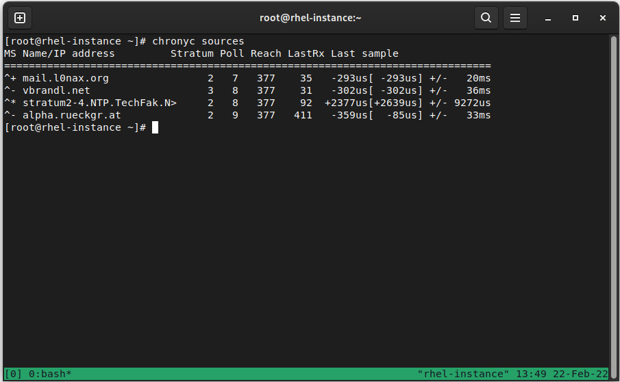
Figure 4.5 – chronyc sources output

As we can see, we know what the status is for each server based on the first column (M), as outlined here:

• ^: This is a server
• =: This is a peer

In the second column (S), we can see the different statuses for each entry, as follows:

• *: This is our current synchronized server
• +: This is another acceptable time source
• ?: This is used to indicate sources that have lost network connectivity
• x: This server is considered a false ticker (its time is considered inconsistent compared to other sources)
• ~: A source that has a high variability (it also appears during daemon startup)

So, we can see that our system is connected to a server that is considering the reference at ts1.sct.de, which is a stratum 2 server.

More detailed information can be checked via the chronyc tracking command, as illustrated in the following screenshot:

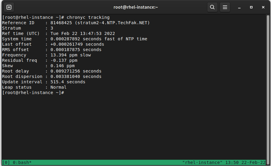
Figure 4.6 – chronyc tracking output

This provides more detailed information about our clock and our reference clock. Each field in the preceding screenshot has the following meaning:

• Reference ID: ID and name/Internet Protocol (IP) address of the server that the system has synchronized.
• Stratum: Our stratum level. In this example, our synchronized server is a stratum 3 clock.
• Ref time (UTC): The last time the reference was processed.
• System time: When running in normal mode (without time skip), this references how far away or behind the system is from the reference clock.
• Last offset: Estimated offset on the last clock update. If it’s positive, this indicates that our local time was ahead of our source.
• RMS offset: Long-term average (LTA) of the offset value.
• Frequency: This is the rate at which the system clock would be wrong if chronyd does not fix it, expressed in parts per million (ppm).
• Residual freq: Reflects any difference between the measurements for the current reference clock.
• Skew: Estimated error on the frequency.
• Root delay: Total network delays to the stratum -1 synchronized server.
• Root dispersion: Total dispersion accumulated through all the computers connected to the stratum -1 server we’re synchronized to.
• Update interval: Interval between the last two clock updates.
• Leap status: This can be Normal, Insert, Delete, or Not synchronized. It reports the leap status.

Tip

Don’t underestimate the information sources you have at your fingertips. Remember that when you’re preparing for Red Hat Certified System Administrator (RHCSA) exams, the information that’s available in the system can be checked during the exam: man pages, documentation included with the program (/usr/share/doc/program/), and more. For example, more detailed information about each field listed here can be found via the man chronyc command.

To configure the client with additional options, other than the ones provided at install time or via the kickstart file, we can edit the /etc/chrony.conf file.

Let’s learn how to convert our system into an NTP server for our network.

NTP server

As we introduced earlier, chrony can also be configured as a server for your network. In this mode, our system will be providing accurate clock information to other hosts without consuming external bandwidth or resources from higher-stratum servers.

This configuration is also performed via the /etc/chrony.conf file, which is where we will be adding a new directive; that is, allow. You can see an illustration of this here:

# Allow NTP client access from all hosts
allow all

This change enables chrony to listen on all host requests. Alternatively, we can define a subnet or host to listen to, such as allow 1.1.1.1. More than one directive can be used to define different subnets. Alternatively, you can use the deny directive to block specific hosts or subnets from reaching our NTP server.

The serving time starts from the base that our server is already synchronized with, as well as an external NTP server, but let’s think about an environment without connectivity. In this case, our server will not be connected to an external source and it will not serve time.

chrony allows us to define a fake stratum for our server. This is done via the local directive in the configuration file. This allows the daemon to get a higher local stratum so that it can serve the time to other hosts. You can see an example of this here:

local stratum 3 orphan

With this directive, we’re setting the local stratum to 3 and we’re using the orphan option, which enables a special mode in which all servers with an equal local stratum are ignored unless no other source can be selected, and its reference ID is smaller than the local one. This means that we can set several NTP servers in our disconnected network, but only one of them will be the reference.

Now that we have covered time synchronization, we are going to dive into resource monitoring. Later, we’ll look at logging. All of this is related to our time reference for the system.

Checking for free resources – memory and disk (free and df)

In this section, you will check the availability of system resources such as memory and disk.

Keeping a system running smoothly means using monitoring so that we can check that the services are running and that the system provides the resources for them to do their tasks.

There are simple commands we can use to monitor the most basic use cases, such as the following ones:

• Disk
• CPU
• Memory
• Network

This includes several ways of monitoring, such as one-shot monitoring, continuously, or even for a period of time to diagnose performance better.

Memory

Memory can be monitored via the free command. It provides details on how much random-access memory (RAM) and swap memory are available and in use, which also indicates how much memory is used by shares, buffers, or caches.

Linux tends to use all available memory; any unused RAM is directed toward caches or buffers and memory pages that are not being used. These are swapped out to disk if available. You can see an example of this here:

# free
              total        used        free      shared  buff/cache   available
Mem:         823112      484884       44012        2976      294216      318856
Swap:       8388604      185856     8202748

In the preceding output, we can see that the system has a total of 823 megabytes (MB) of RAM and that it’s using some swap and some memory for buffers. This system is not swapping heavily as it’s almost idle (we’ll check the load average later in this chapter), so we should not be concerned about it.

When RAM usage gets high and there’s no more swap available, the kernel includes a protection mechanism called Out-of-Memory Killer (OOM Killer). It determines— based on time in execution, resource usage, and more—which processes in the system should be terminated to recover the system so that it’s functional. This, however, comes at a cost, as the kernel knows about the processes that may have gone out of control. However, the killer may kill databases and web servers and leave the system in an unstable state. For production servers, it is sometimes typical—instead of letting the OOM-Killer start killing processes in an uncontrolled way—to either tune the values for some critical process so that those are not killed or to cause a system crash.

A system crash is used to collect debug information that can later be analyzed via a dump containing information about what caused the crash, as well as a memory dump that can be diagnosed.

We will come back to this topic in Chapter 16, Kernel Tuning and Managing Performance Profiles with tuned. Let’s move on and check the disk space that’s in use.

Disk space

Disk space can be checked via the df tool. df provides data as output for each filesystem. This indicates the filesystem and its size, available space, percent of utilization, and mount point.

Let’s check this in our example system, as follows:

# df

Filesystem            1K-blocks     Used Available Use% Mounted on

devtmpfs                 442628        0    442628   0% /dev

tmpfs                    489100        0    489100   0% /dev/shm

tmpfs                    195640     5380    190260   3% /run

/dev/mapper/rhel-root  40935908 18334816  22601092  45% /

/dev/sda2               1038336   565624    472712  55% /boot

/dev/sda1                102182     7704     94478   8% /boot/efi

By using this, it’s easy to focus on filesystems with higher utilization and less free space to prevent issues.

Important Note

If a file is being written, such as by a process logging its output, removing the file will just unlink the file from the filesystem, but since the process still has the file handle open, the space is not reclaimed until the process is stopped. In case of critical situations where disk space must be made available as soon as possible, it’s better to empty the file via a redirect, such as echo "" > filename. This will recover the disk space immediately while the process is still running. Doing this with the rm command will require the process to be finalized.

We’ll check out CPU usage next.

CPU

When it comes to monitoring the CPU, we can make use of several tools, such as ps. You can see this in use here:

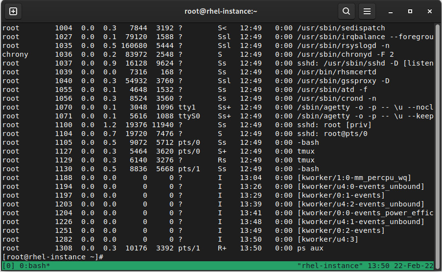
Figure 4.7 – Output of the ps aux command (every process in the system)

The ps command is the de facto standard for checking which process is running, as well as resource consumption usage.

As for any other command, we could write a lot about all the different command arguments we could use (so, again, check the man page for details), but as a rule, try to learn about their basic usage or the ones that are more useful for you. For anything else, check the manual. For example, ps aux provides enough information for normal usage (every process in the system).

The top tool, as shown in the following screenshot, refreshes the screen regularly and can sort the output of running processes, such as CPU usage, memory usage, and more. In addition, top also shows a five-line summary of memory usage, load average, running processes, and so on:

Figure 4.8 – top execution on our test system

CPU usage is not the only thing that may keep our system sluggish. Now, let’s learn a bit about load average indicators.

Load average

Load average is usually provided as a group of three numbers, such as load average: 0.81, 1.00, 1.17, which is the average that’s calculated for 1, 5, and 15 minutes, respectively. This indicates how busy a system is; the higher it is, the worse it will respond. The values that are compared for each time frame give us an idea of whether the system load is increasing (higher values in 1 or 5 and lower on 15) or if it is going down (higher at 15 minutes, lower at 5 and 1), so it becomes a quick way to find out if something happened or if it is ongoing. If a system usually has a high load average (over 1.00 per CPU), it would be a good idea to dig a bit deeper into the possible causes (too much demand for its power, not many resources available, and so on).

Now that we have covered the basics, let’s move on and look at some extra checks we can perform on our system resources’ usage.

Other monitoring tools

For monitoring network resources, we can check the packages that are sent/received for each card via ifconfig (installed via the net-tools package), for example, and match the values that are received for transmitted packages, received packages, errors, and so on.

When the goal is to perform more complete monitoring, we should ensure that the sysstat package is installed. It includes some interactive tools such as iostat, which can be used to check disk performance, but the most important thing is that it also sets up a job that will collect system performance data on a periodical basis (the default is every 10 minutes). This will be stored in /var/log/sa/.

Historical data that’s recorded and stored per day (##) at /var/log/sa/sa## and /var/log/sa/sar## can be queried so that we can compare it against other days. By running the data collector (which is executed by a systemd timer) with a higher frequency, we can increase the granularity for specific periods while an issue is being investigated.

However, it appears the sar file is showing lots of data, as we can see here:

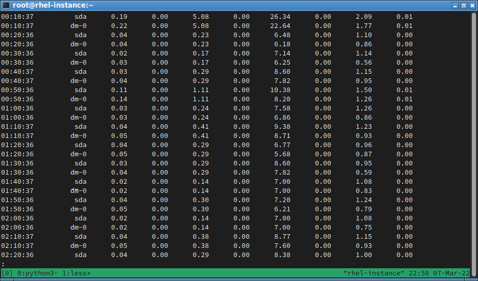
Figure 4.9 – Contents of /var/log/sar02 on the example system

Here, instead of seeing sda, we might see references to devices such as 8-0. In this case, the device’s name is using the values for the major/minor, which we can check in the /dev/ folder. We can see this by running ls -l /dev/*|grep 8, as shown in the following screenshot:

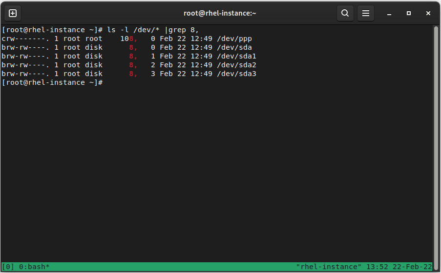
Figure 4.10 – Directory listing for /dev/ for locating the device corresponding to major 8 and minor 0

Here, we can see that this corresponds to the full hard-drive statistics at /dev/sda.

Tip

Processing the data via sar is a good way to get insights into what’s going on with our system, but since the sysstat package has been around for a long time in Linux, there are tools such as sarstats (https://github.com/mbaldessari/sarstats) that help us process the data that’s recorded and present it graphically as a Portable Document File (PDF) file.

In the following screenshot, we can see the system service times for the different drives, along with a label at the time the system crashes. This helps us identify the system’s activity at that point:

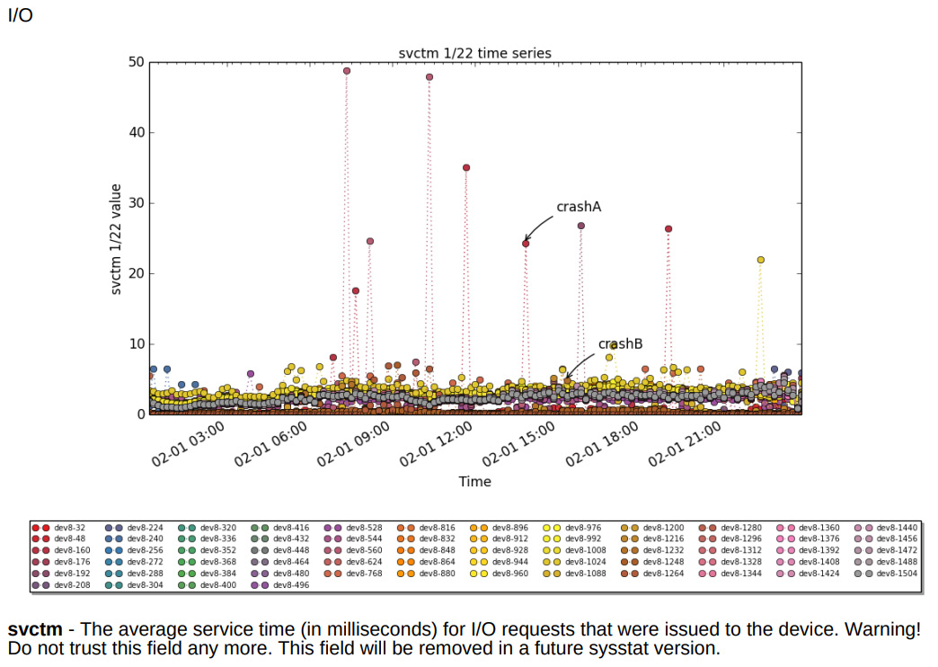
Figure 4.11 – sarstats graphics for the disk service’s time in the example PDF at https://acksyn.org/software/sarstats/sar01.pdf

Modern tooling for monitoring the system’s resources has evolved, and Performance Co-Pilot (pcp and, optionally, the pcp-gui package) can be set up for more powerful options. Just bear in mind that pcp requires us to also start the data collector on the system.

RHEL 9 also includes Cockpit, which is installed by default when we do a server installation. This package provides a set of tools that enable web management for the system, and it can also be made part of other products via plugins that extend its functionality.

The web service provided by Cockpit can be reached at your host IP at port 9090, so you should access https://localhost:9090 to get a login screen so that we can use our system credentials to log in.

Important Tip

If Cockpit is not installed or available, make sure that you execute dnf install cockpit to install the package and use systemctl enable --now cockpit.cocket to start the service. If you are accessing the server remotely, instead of using localhost, use the server hostname or IP address after allowing the firewall to connect via firewall-cmd --add-service=cockpit, if you haven’t done so previously.

After logging in, we will see a dashboard showing the relevant system information and links to other sections, as shown in the following screenshot:

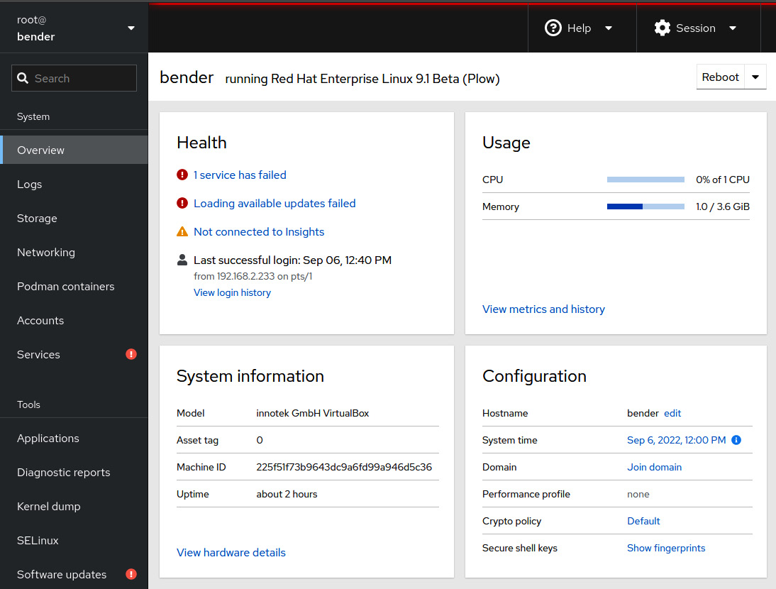
Figure 4.12 – Cockpit screen after logging in with a system dashboard

As you can see, Cockpit includes several tabs that can be used to view the status of the system and even perform some administration tasks, such as Security-Enhanced Linux (SELinux) tasks, software updates, subscriptions, and more.

For example, we can check the system graphs on performance, as shown in the following screenshot:

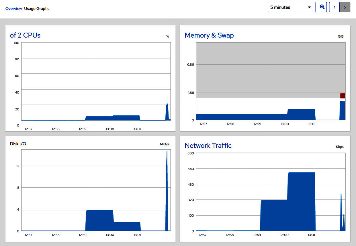
Figure 4.13 – Cockpit graphs in Usage Graphs dashboard

Cockpit allows us to check a service’s status and package upgrade status, plus other configuration settings from a graphical interface that can also connect remotely to other systems. These can be selected from the lateral menu on the left.

There are better tools suited for large deployment monitoring and management, such as Ansible and Satellite, so it is important to get used to the tools we have for troubleshooting and simple scripts we can build. This allows us to combine what we’ve learned so far to quickly generate hints about things that require our attention.

With that, we have covered some of the basics of checking resource usage. Now, let’s check out how to find information about the running services and errors we can review.

Finding logs, using journald, and reading log files, including log preservation and rotation

In this section, you will learn how to review a system’s status via logs.

Previously in this chapter, we learned how to manage system services via systemd, check their status, and check their logs. Traditionally, the different daemons and system components used to create files under the /var/log/ folder are based on the name of the daemon or service. If the service is used to create several logs, it would do so inside a folder for the service (for example, httpd or samba).

The rsyslogd system log daemon has a new systemd partner—named systemd-journald.service—that also stores logs, but instead of using the traditional plain text format, it uses the binary format, which can be queried via the journalctl command.

It’s really important to get used to reading the log files as it’s the basis for troubleshooting, so let’s learn about general logging and how to use it.

Logs contain status information for the services that generate them. They might have some common formatting and can often be configured, but they tend to use several common elements, such as the following:

• Timestamp
• Module generating the entry
• Message

Here is an example:

Jan 03 22:36:47 rhel-instance sshd[50197]: Invalid user admin from 49.232.135.77 port 47694

In this case, we can see that someone attempted to log in to our system as the admin user from IP address 49.232.135.77.

We can correlate that event with additional logs, such as the ones for the login subsystem via journalctl -u systemd-logind. In this example, we cannot find any login for the admin user (this is expected, as the admin user was not defined in this system).

Additionally, we can see the name of the host (rhel-instance), the service generating it (sshd), a PID of 50197, and the message that’s been logged by that service.

In addition to journalctl, there are additional logs that we can look at when we wish to check the system’s health. Let’s look at an example with /var/log/messages:

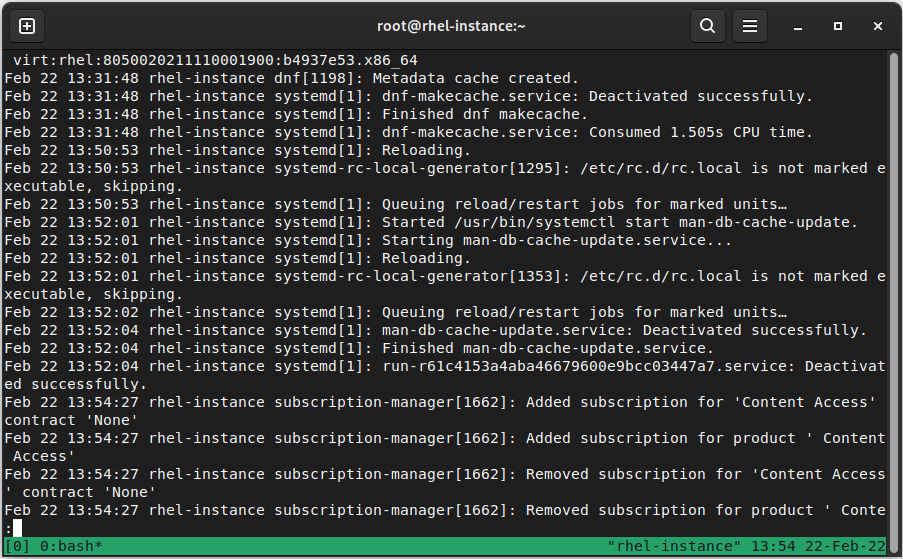
Figure 4.14 – Excerpt of /var/log/messages

In this example, we can see how the system ran some commands while following a similar output to the initial lines. For example, in the preceding example, we can see how sysstat has been executed every 10 minutes, as well as how the dnf cache has been updated.

Let’s look at a list of important logs that are available in a standard system installation (note that the filenames are relative to the /var/log folder):

• boot.log: Stores the messages that are emitted by the system during boot. It might contain escape codes that are used to provide colorized output.
• audit/audit.log: Contains the stored messages that have been generated by the kernel audit subsystem.
• secure: Contains security-related messages, such as failed sshd login attempts.
• dnf.log: Logs generated by the Dandified YUM (DNF) package manager, such as cache refreshes.
• firewalld: Output generated by the firewalld daemon.
• lastlog: This is a binary file that contains information about the last few users logging in to the system (to be queried via the last command).
• messages: The default logging facility. This means that anything that is not a specific log will go here. Usually, this is the best place to start checking what happened with a system.
• maillog: The log for the mail subsystem. When enabled, it attempts to deliver messages. Any messages that are received will be stored here. It’s common practice to configure outgoing mail from servers so that system alerts or script outputs can be delivered.
• btmp: Binary log for failed access to the system.
• wtmp: Binary log for access to the system.
• sa/sar*: Text logs for the sysstat utility (the binary ones, named sa, plus the day number, are converted via a cron job at night).

Additional log files might exist, depending on the services that have been installed, the installation method that was used, and so on. It is very important to get used to the available logs and—of course—review their contents to see how the messages are formatted, how many logs are created every day, and what kind of information they produce.

Using the information that’s been logged, we will get hints on how to configure each individual daemon. This allows us to adjust the log level between showing just errors or being more verbose about debugging issues. This means we can configure the required log rotation to avoid risking system stability because all the space has been consumed by logs.

Log rotation

During regular system operation, lots of daemons are in use, and the system itself generates logs that are used for troubleshooting and system checks.

Some services might allow us to define a log file to write to based on the date, but usually, the standard is to log to a file named like the daemon in the /var/log directory; for example, /var/log/cron. Writing to the same file will cause the file to grow until the drive holding the logs is filled, which might not make sense as after a while (sometimes, under company-defined policies), logs are no longer useful.

The logrotate package provides a script with a cron entry that simplifies the log rotation process. It is configured via /etc/logrotate.conf and is executed on a daily basis, as shown here:

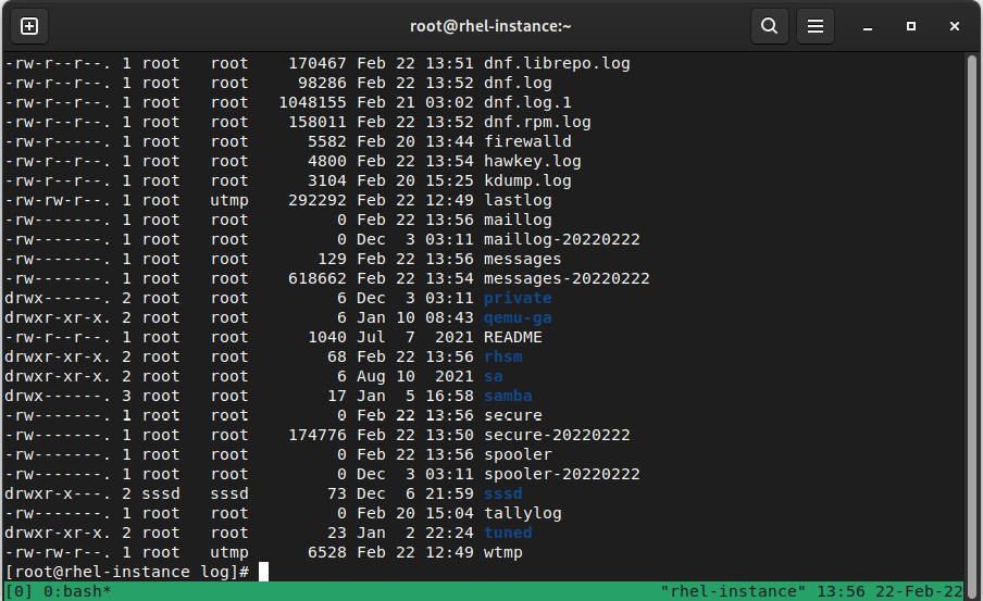
Figure 4.15 – Example listing of logs and rotated logs (using date extension)

If we check the contents of the configuration file, we will see that it includes some file definitions either directly there or via drop-in files in the /etc/logrotate.d/ folder, which allows each program to drop its own requirements without it affecting others when packages are installed, removed, or updated.

Why is this important? Because—if you remember from some of the tips earlier in this chapter (while speaking about disk space)—if logrotate just deleted the files and created a new one, the actual disk space would not be freed, and the daemon writing to the log would continue to write to the file it was writing to (via the file handle). To overcome this, each definition file can define a post-rotation command. This signals the process of log rotation so that it can close and then reopen the files it uses for logging. Some programs might require a signal such as kill –SIGHUP PID or a special parameter on execution, such as chronyc cyclelogs.

With these definitions, logrotate will be able to apply the configuration for each service and, at the same time, keep the service working in a sane state.

The configuration can also include special directives, such as the following:

• missingok
• nocreate
• copytruncate
• notifempty

You can find out more about them (and others) on the man page for logrotate.conf (yes—some packages also include a man page for the configuration files, so try checking man logrotate.conf to get the full details!).

The remaining general configuration in the main file allows us to define some common directives, such as how many days of logs to keep, if we want to use the date in the file extension for the rotated log files, if we want to use compression on the rotated logs, how frequently we want to have the rotation executed, and so on.

Let’s look at some examples.

The following example will rotate on a daily basis, keep 30 rotated logs, compress them, and use an extension with date as part of its trailing filename:

rotate 30
daily
compress
dateext

In this example, it will keep 4 logs rotated on a weekly basis (so 4 weeks) and will compress the logs, but use a sequence number for each rotated log (this means that each time a rotation happens, the sequence number is increased for the previously rotated logs too):

rotate 4
weekly
compress

One of the advantages of this approach (not using dateext) is that the log naming convention is predictable as we have daemon.log as the current one, daemon.1.log as the prior one, and so on. This makes it easier to script log parsing and processing.

Summary

In this chapter, we learned about systemd and how it takes care of booting the required system services in an optimized way. We also learned how to check a service’s status, how to enable, disable, start, and stop it, and how to make the system boot into the different targets that we boot our system into.

Time synchronization was introduced as a must-have feature, and it ensures our service functions properly. It also allows us to determine the status of our system clock and how to act as a clock server for our network.

We also used system tools to monitor resource usage, learned how to check the logs that are created by our system to find out about the functional status of the different tools, and how we can ensure that logs are maintained properly so that older entries are discarded when they are no longer relevant.

In the next chapter, we will dive into securing the system with different users, groups, and permissions.