The term ‘photovoltaics’ comes from two words, ‘photo’ and ‘Volta’; photo stands for light and comes from the Greek phõs, or photós. The Italian physicist Alessandro Giuseppe Antonio Anastasio Count Volta, who was born in 1745, was the inventor of the battery and together with Luigi Galvani is considered to have discovered electricity. There is not much that associates him with photovoltaics. However, in 1897, 70 years after Volta's death, the measurement unit for electric voltage was named volt in his honour. Photovoltaics, or PV for short, therefore stands for the direct conversion of sunlight into electricity.
While experimenting with electro-chemical batteries with zinc and platinum electrodes, the 19-year-old Frenchman Alexandre Edmond Becquerel found that the electric voltage increased when he shone a light on them. In 1876 this phenomenon was also proven with the semiconductor selenium. In 1883 the American Charles Fritts produced a selenium solar cell. Due to the high prices of selenium and manufacturing difficulties, this cell was not ultimately used to produce electricity. At the time, the physical reason why certain materials produce electric voltage when radiated with sunlight was not understood. It was not until many years later that Albert Einstein was able to specify the photo effect that causes this. He eventually received the Nobel Prize for this work in 1921.
The age of semiconductor technology began in the mid-1950s. The abundant semiconductor material (see info box in the next section.) silicon became all the rage in technology, and in 1954 the first silicon solar cell made its appearance at American Bell Laboratories. This was the basis for the successful and commercial further development of PV.
5.1 Structure and Function
5.1.1 Electrons, Holes, and Space-Charge Regions
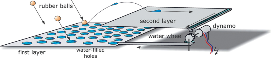
Understanding the relatively complicated way that solar cells work requires immersion into the most extreme depths of physics, but the small applied model shown in Figure 5.1 roughly explains the principle involved. There are two horizontal levels. The second level is located slightly higher than the first one. The first level has a large number of small hollows filled to the top with water. The water here cannot move by itself. Now someone starts to throw small rubber balls at the first level. If a ball hits a hole, the water splashes upwards and ends up on the second level. Here there are no hollows to contain the water. The second level is therefore inclined so that the water runs off and reaches the draining groove on its own. This groove is connected to the second level through a pipe and as the water flows through, it drives a small waterwheel with a dynamo. When the water reaches the lower level, it fills up the hollows again. The cycle can start all over again with new rubber balls.
Figure 5.1 Model illustrating the processes of a solar cell.
However, we want to use solar cells not to produce a water cycle but to generate electric current to run electrical appliances. Electric current is created from the flow of negative charge carriers, called electrons. These are the same as the water in our simple model. The solar cell needs a material with two levels: one level where the electrons are firmly fixed, like the water collecting in the hollows, and a second level where the electrons are able to move freely. Semiconductor materials normally have precisely these properties. Tiny particles of light, called photons in physics, correspond to the rubber balls and are able to raise the electrons to the second level.
Conductors, Non-conductors, and Semiconductors
Conductors such as copper always conduct electric current relatively well, but non-conductors such as plastics conduct almost no electricity at all. In contrast, semiconductors – as the name indicates – only conduct electric current sometimes, for example at high temperatures, when fed with electric voltage or when radiated with light. These effects are used in the production of electronic switches like transistors, computer chips, special sensors and even solar cells.
Organic semiconductors are available in addition to elementary semiconductors, such as silicon (Si), and compound semiconductors, such as gallium arsenide (GaAs), Cadmium telluride (CdTe), and copper indium diselenide (CuInSe2). All these materials are used in PV.
The tilt in our simple model is important, because it enables the cycle to function perfectly. Otherwise the water will not collect on its own in the rain gutter. With semiconductors the second level must also have an incline that enables the electrons to gather on one side. In contrast to our simple model, it is not gravity that is used to collect the electrons but instead an electric field, which pulls the negatively charged electrons to one side. To produce this field, the semiconductor is ‘doped’. One side of the semiconductor is deliberately contaminated with an element like boron and the other side with a different element like phosphorus. As boron and phosphorus also have a varying number of electrons, they produce the necessary incline. The crossing area is called a space-charge region. An electric field is created here, which pulls the electrons to one side. There, external contacts collect them and they flow back to the first level through an external electric circuit. In the process they produce electrical energy.
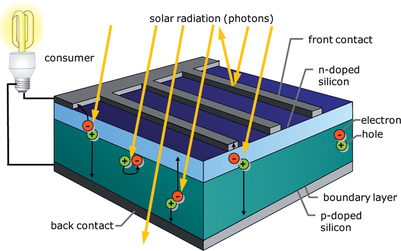
Figure 5.2 shows the principal structure of a silicon solar cell. In technical jargon the different doped sides of the silicon wafer are called n-doped and p-doped silicon, respectively. Between the two areas is a barrier layer with the space-charge region. Light in the form of photons separates negatively charged particles (electrons) and positively charged particles (holes) and ensures that the electrons are able to move about freely at the second level. In contrast to the simple model shown, the holes also move. The electrons and holes are separated by the space-charge region. Thin front contacts collect the electrons on the front side of the cell.
Figure 5.2 Structure and processes of a solar cell [Qua13].
However, not every light particle ensures that an electron is separated from the hole. If the energy of the photon is too low, the electron will fall back into the hole. On the other hand, if the energy of the photon is too high, only part of it is used to separate the electron from the hole. Some photons also move through the solar cell unused; others are reflected by the front contacts.
5.1.2 Efficiency, Characteristics, and MPP
The efficiency of the solar cell describes what proportion of the solar radiation power the cell converts into electrical power.
Solar Cell Efficiency
The higher the efficiency, the more electric power the solar cell can generate per square metre. In addition to the type of materials used, the quality of the manufacturing also plays a major role. Today silicon cells in mass production reach a maximum efficiency of almost 24%. More than to 25% efficiency has already been reached in laboratories (Table 5.1).
Incidentally, conventional petrol engines do not reach a level of efficiency higher than silicon cells. Compared to the 5% efficiency of the first solar cells in 1954, technology has advanced considerably. If individual solar cells are packaged into PV modules, the efficiency drops somewhat due to the space necessary between the cells and the module frames. It is hoped that, in the future, other materials can be used to produce further cost savings. Compared to silicon cells, however, the efficiencies still need to be improved. Concentrator cells in which sunlight is concentrated through mirrors or lenses reach a very high efficiency but are considerably more expensive than normal silicon cells.
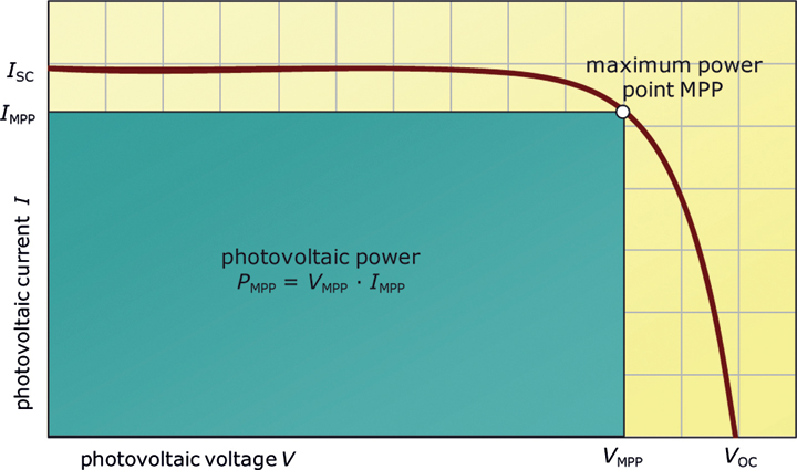
In addition to efficiency, there are other parameters that describe PV modules. Data sheets for PV modules usually contain a current-voltage characteristic curve. The maximum current IK flows with a short-circuited PV module. The short-circuiting is harmless for the module. The short-circuit current is limited and depends on the solar radiation intensity, also referred to as irradiance. If nothing is connected to the PV module, it is in open-circuit state and no current flows. In this case it adjusts itself to the open-circuit voltage VOC. A PV module is unable to produce any power when in short-circuit or open-circuit state. Between open-circuit and short-circuit state, the current depends on the voltage. The basic characteristic curve is similar for all solar modules (Figure 5.3).
Figure 5.3 Current-voltage characteristic curve of a PV module.
In practice, the aim is to extract the maximum power from the PV module. This corresponds to the largest rectangle that can be fitted under the characteristic curve. The upper right edge of the rectangle on the characteristic curve is called maximum power point or MPP. The corresponding voltage is called MPP voltage or VMPP for short. At this voltage, the PV module delivers the maximum power. In practice, operation near the MPP can be achieved by connecting a battery whose voltage is close to the MPP voltage, for example, or by using an inverter that automatically adjusts the MPP voltage on the PV module.
The current of PV module, and hence the power, decreases according to the number of incoming photons, i.e. the irradiance of the sunlight. For example, if the solar irradiance drops by 50%, the output of the PV module also drops by 50%. The output of PV modules also drops at high temperatures. If the temperature rises by 25 °C, the output of crystalline solar cells drops by around 10%. Therefore, when installing PV modules, care should be taken to ensure they are always well-ventilated and a draft of air cools the modules.
Standard test conditions (STCs) for comparing PV modules have been agreed internationally. The MPP power of solar cells and modules is determined at a solar irradiance of 1000 W per m2 and a module temperature of 25 °C. Since in practice the irradiance is usually lower and PV modules can heat up to over 60 °C in summer, the MPP power determined under STCs represents a maximum value. This value is only achieved rarely and exceeded even less frequently. For this reason, the unit ‘Watt Peak’, Wp for short, is also used (Table 5.2).
Voltage of a PV module in open-circuit state without connected load
Short-circuit current
ISC
Ampere, A
Current of a PV module in short-circuit state
MPP voltage
VMPP
Volt, V
Voltage at which a PV module delivers maximum power
MPP current
IMPP
Ampere, A
Current associated with the MPP voltage
MPP power
PMPP
Watt, W
Maximum power a PV module can deliver
5.2 Production of Solar Cells – From Sand to Cell
5.2.1 Silicon Solar Cells – Power from Sand
Silicon, the raw material for computer chips and solar cells, is the second most common element in the Earth's crust after oxygen. However, in nature silicon occurs almost exclusively as an inclusion in quartz sand or silicate rock, or as silicic acid in the world's oceans. Even the human body contains around 20 mg of silicon per kilogram of body weight.
Pure silicon, on the other hand, is usually obtained from quartz sand. Chemically, quartz sand is pure silicon dioxide (SiO2). To obtain silicon from it, the oxygen atoms (O2) have to be separated at high temperatures. This process is called reduction and is carried out in arc furnaces, for example, at temperatures of around 2000 °C. The result is industrial raw silicon with a purity of 98–99%.
Raw silicon has to be purified further before it can be used to produce solar cells. The Siemens process is usually used for this purpose. Hydrogen chloride is used to convert the raw silicon into trichlorosilane, which is then distilled. At high temperatures of 1000–1200 °C the silicon is then separated again into long rods. The resulting polycrystalline solar-grade silicon has a purity of over 99.99% (Figure 5.4).
Figure 5.4 Polycrystalline silicon for solar cells. Left: Raw silicon. Centre: Silicon blocks. Right: Silicon wafers.
Source: Photos: PV Crystalox Solar plc.
The silicon is melted down again to produce semiconductor silicon for computer chips and monocrystalline solar cells. In the crucible process invented by Polish chemist Jan Czochralski, a crystal seed is dipped into a crucible with a silicon melt and then slowly pulled upwards in a rotating movement. The molten silicon attaches itself to the crystal and a long, round silicon rod is created. In the process the silicon crystals align in one direction. This creates monocrystalline silicon. Most of the impurities remain in the melting crucible so that the semiconductor silicon is left with purities of over 99.9999%.
In the next step, wire saws cut the long silicon rods into thin slices, called wafers. This sawing process results in significant waste, with up to 50% of the valuable silicon material being lost as a result. The alternative is for two thin wires to be pulled through the liquid silicon melt. With this procedure, thin silicon wafers are formed between the two wires. Immersion in acid will remove sawing damage from wafers and smooth the surfaces. Several years ago, silicon wafers had a thickness of 0.3–0.4 mm. Nowadays, in order to save material and costs, the wafer thickness is reduced to well below 0.2 mm. This used to be a major technical challenge, since the ultra-thin wafers must not break apart.
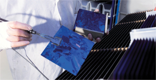
The finished wafers are exposed to gaseous doping substances referred to as dopants. This produces the p- and n-layers described earlier. A transparent anti-reflection layer of silicon nitride less than a millionth of a millimetre thick gives the silicon solar cell its typical dark blue colour. This layer reduces the reflection loss of the silver-grey silicon on the front side of the solar cell. The darker the cell appears, the less light it reflects (Figure 5.5).
Figure 5.5 Polycrystalline solar cells with anti-reflective coating before the front contacts are applied.
The front and back contacts are then applied using screen printing. To reduce the losses at the opaque front contacts, some manufacturers conceal them under the surface or try to move them to the back of the cell. Although this increases the efficiency of cells, it is also a more complicated and expensive way to manufacture them. The finished cells are then tested and sorted according to performance classes for further processing into PV modules.
5.2.2 From Cell to Module
Silicon solar cells are usually square in shape. The length of the edge is measured in inches. Originally, solar cells were typically 4 in. (approx. 10 cm) in length. Meanwhile, a measurement of 6 in. (approx. 15 cm) has established itself as the standard. Some manufacturers are already producing 8-in. (approx. 20 cm) solar cells. Large solar cells require fewer processing steps to be made into modules. However, there is greater risk that the cells will break during further processing. The current increases with the size of a solar cell, whereas the voltage remains constant. The electric voltage of a solar cell is only 0.6–0.7 V.
Clearly, higher voltages are needed for practical applications. Therefore, many cells are interconnected in series to form solar modules. Soldered wires are used to connect the front contacts of a cell to the back contacts of the next cell. It takes 32–40 cells connected in series to produce a voltage high enough to charge 12-V batteries. Higher voltages are needed to feed into the grid through inverters. Solar modules with at least 60 cells connected in series are common for this purpose.
Solar cells are very sensitive, break easily, and corrode when in contact with moisture, so they must be protected. Consequently, they are embedded in a layer of special plastic between the front glass panel and a plastic film on the back (Figure 5.6). Some manufacturers also use glass for the back. The glass provides mechanical stability and must be very translucent. The plastic material used for embedding the solar cells consists of two thin films of ethylene-vinyl acetate (EVA). At temperatures of around 100 °C these films bond with the cells and the glass. This process is called lamination. The finished laminate then protects the cells from the effects of the weather, especially moisture.
Figure 5.6 Basic structure of a photovoltaic module.
The connections of the solar cells are linked to a module junction box. Individual faulty cells or uneven shade can damage a PV module. Bypass diodes are designed to prevent any damage by compensating for any faulty cells. These diodes are also usually integrated into the module junction boxes.
5.2.3 Thin-Film Solar Cells
Crystalline solar cells are practically carved from solid blocks, a process which requires a comparatively large amount of costly semiconductor material. Alternative production methods using thin-film cells seek to reduce the amount of material needed. Whereas crystalline solar cells reach thicknesses in the order of tenths of millimetres, the thickness of thin-film solar cells is in the thousandths of a millimetre range. The production principle is similar even when different materials such as amorphous silicon (a-Si), cadmium telluride (CdTe), or copper indium diselenide (CIS) are used (Figure 5.7).
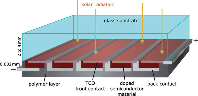
Figure 5.7 Cross-section of a thin-film PV module.
The base of thin film solar cells is a substrate that is usually made of glass. Plastic can be used instead of glass for the substrate to produce modules that are flexible and bendable. A thin TCO (Transparent Conductive Oxide) layer is applied to the substrate using a spraying technique. A laser or micro-cutter then separates this layer into strips. The individual strips constitute the single cells that form the basis of the solar module. Like crystalline cells, these cells are also bonded in such a way that they are connected in series to increase the electric voltage. The long strips make it visually easy to distinguish thin-film modules from crystalline solar modules.
The semiconductor and doping materials are then vaporized at high temperatures. When silicon is vaporized as a semiconductor material, its crystalline structure is lost. This is referred to as amorphous silicon. A screen-printing procedure then applies materials like aluminium to the contact at the back. A layer of polymer seals the cell at the back to protect it from moisture.
The efficiency of thin-film modules is currently still lower than that of crystalline PV modules. This means that a larger surface is required for the same power output, and, therefore, more assembly is required, and the associated costs are higher. However, the efficiency of individual thin-film technologies has increased significantly in recent years. Nevertheless, thin-film technology has not succeeded in breaking the dominance of crystalline solar modules.
In addition to thinfilm materials, other technologies are currently being tested. Pigment cells and organic solar cells could eventually offer a cost-effective alternative to present-day technologies. At the moment it is almost impossible to predict which technologies will prove to be the best in 30 or 40 years' time. The fact is that competition stimulates business, and costs will continue to fall due to the rivalry between different PV technologies.
5.3 PV Systems – Grids and Islands
5.3.1 Sun Islands
With PV systems a distinction is made between stand-alone (island) systems and grid-coupled systems. Stand-alone solar systems work autonomously without being connected to an electricity grid. For example, they are often used in small applications, such as wristwatches and pocket calculators. This is because, in the long run, they are less expensive than using disposable batteries to supply energy, and a network cable in this case would be highly impractical. Stand-alone solar systems are also popular for use in small systems like car park ticket machines. In this case it is less expensive to install a PV system than to lay network cables and install a metre (Figure 5.8).
Figure 5.8 Stand-alone PV systems offer advantages for many applications compared to grid connections.
However, the big market for solar stand-alone systems is in areas that are far from an electricity grid. Globally, around two billion people have no access to electricity. Even in industrialized countries there are towns that are very remote from the grid and where any kind of cabling would be extremely expensive. There are alternatives to using stand-alone solar systems, such as diesel generators. However, nowadays a solar system often compares favourably in terms of cost and supply reliability, especially in cases with low electricity demand. Nevertheless, the capital costs of stand-alone PV systems are relatively high. Diesel generators are cheaper to buy. However, due to the high cost of diesel fuels, they are usually more expensive than the solar alternative over their entire service life. In developing countries in particular, special financing models such as microcredits can help to overcome the hurdle of high capital costs and thus promote the further spread of PV.
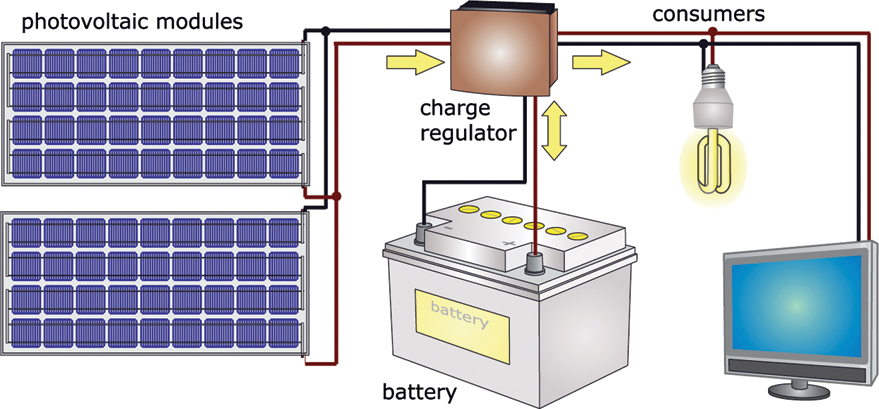
Solar island systems are comparatively straightforward and can even be installed by people with limited technical skills (Figure 5.9). A battery ensures that supply is available at night or during periods of bad weather. For reasons of cost, lead batteries are normally used. In principle, 12-V car batteries are also an option. Special-purpose solar batteries have a considerably longer lifetime, but are also more expensive. Since batteries can quickly be ruined as a result of leakage or overcharging, a charge regulator protects the battery. The battery, the power consumer, and the PV module are connected directly to the charge controller. Take care not to mix up the positive and negative poles; otherwise a short circuit may occur.
When the battery is nearly empty, the consumer load is switched off. Although the loss of power is annoying, this is better than a defective battery. Once the battery reaches a certain charge level again, the charge controller automatically switches the consumer load back on. Once the battery is fully charged, the charge controller separates the PV module and prevents the battery from overloading.
The costs can be kept low if the consumer loads are energy-efficient. A battery voltage higher than 12 V is recommended for consumers with higher loads, as otherwise the losses in the lines will be too high. Island systems work on a direct-current (DC) voltage basis, so, if possible, only DC consumer loads should be used. Special 12 or 24 V DC refrigerators, lamps, and entertainment devices are available. To use alternating current (AC) consumers, a stand-alone inverter must first convert the DC voltage of the battery to AC voltage.
Normal low voltages are relatively safe, at least as far as contact is concerned. Since batteries are power packs, improper handling can cause short circuits, fire, or even explosions. Battery rooms should always have good ventilation as hydrogen gas can build up in them. Lead batteries contain diluted acid. Over time, water evaporates from the battery, and the battery must be refilled regularly. With maintenance-free batteries the water is bound in a gel and cannot escape.
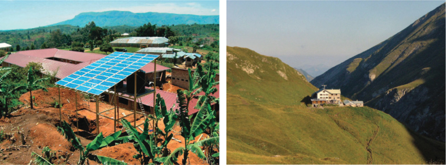
A large array of PV modules can end up costing the same as a mid-range car, and even individual PV modules are quite expensive, so thieves are making life increasingly difficult for the operators of remote PV systems. Solar modules installed on quiet roads are particularly vulnerable to theft. Since stand-alone systems are usually installed in less busy locations, the risk of theft is especially high. This risk should be minimized during installation. Ideally, PV systems should not be visible from public roads. However, if this cannot be avoided, systems should at least be installed in places that are difficult to access (Figure 5.10).
Figure 5.10 Typical locations for stand-alone PV systems. Left: Electricity supply for a village in Uganda. Right: Alpine lodge.
Source: SMA Technologie AG.
In Germany, small solar systems can only make a small contribution to climate protection. Nevertheless, PV-based pocket calculators and watches help reduce the mountain of small spent batteries. In countries with poorly developed electricity grids, however, stand-alone PV systems are becoming increasingly attractive as an alternative to diesel generators, which have dominated until now, and can play an important role in the climate-friendly development of electricity supply systems.
5.3.2 Sun in the Grid
PV systems that feed into the public grid are built in a different way from island systems. First of all, they normally require a larger number of modules. Crystalline solar modules installed over a 30 m2 area can yield a peak output of 4–5 kWp. In Germany this generates between 3500 and 5000 kWh with the right kind of roof; in Southern Europe or good sites in the USA the figure increases by around 50%. This can easily cover the electricity demand of an average household. An ideal surface can usually be found on the roofs of single-family houses.
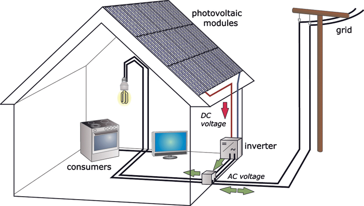
Since solar modules deliver DC voltage, but the public grid works with AC voltage, an inverter is required. An inverter converts the DC voltage of a PV module to AC voltage. Modern inverters have high demands placed on them. They are required to have a high level of efficiency to ensure that, any loss of valuable solar energy resulting from conversion into AC voltage is minimal. Modern PV inverters achieve efficiencies of up to 98%. It is important that the efficiency is also high under partial load, i.e. cloudy skies. European efficiency describes average inverter efficiency based on Central European climate conditions, while CEC efficiency is for Californian conditions (Figure 5.11).
Figure 5.11 The principle of a grid-connected PV system.
Inverters also have to monitor the grid constantly and switch off the solar feed when a general grid outage occurs. Otherwise, if the electricity supply company wants to carry out work on the grids and switch off the power for this purpose, the solar power fed into the grid could endanger the workers. If a public power outage occurs, owners of PV systems will unfortunately end up sitting in the dark even though there is nothing wrong with their solar system. Technically, a solar system can be kept running in island mode, using batteries, if the grid fails. This option will be described in more detail later.
An inverter does not only convert voltage. It also ensures that PV modules operate with the optimal voltage and deliver the maximum possible power. The optimal voltage setting is referred to as MPP tracking. At the system design stage, it is important to match the number of PV modules to the inverter. The leading inverter manufacturers usually offer relevant design software free of charge.
Shadowing can also cause problems. PV systems react sensitively, and performance suffers even if only part of a system is in the shade. If three cells are in shade, the entire PV module can stop working. Therefore, a site that has minimal shade is more important for the installation of a system than an optimal orientation towards the sun.
Grid-connected PV systems feed all the electricity they generate into the public grid. They act as solar power plants. Solar systems can also track the sun (Figure 5.12). Systems that use tracking can increase power output by 30% on average over the year. However, tracking also increases the capital cost and requires additional maintenance due to the mechanical parts required. Since module prices have fallen sharply in recent years, tracking systems are quite rare these days.
Figure 5.12 The ‘Gut Erlasee’ tracked solar power plant in Bavaria, Germany, has a total output of 12 MW.
Source: SOLON SE, Photo: paul-langrock.de.
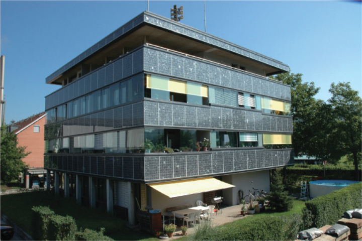
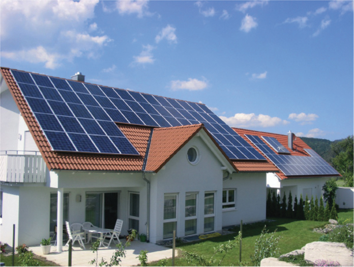
The neatest looking installations of PV systems are those on roofs and façades (Figures 5.13 and 5.14). Less building material is needed for this type of installation, which is a cost advantage of PV systems. And compared to a representative marble façade, PV is now available at a bargain price.
Some of the solar power can be used directly in the building when the system is installed. If the PV system produces more power than the building needs, it feeds the surplus electricity into the public grid. If the output of the solar system is not sufficient to cover the building's own requirements, the electricity shortfall is taken from the grid. In a sense, the grid acts as a storage unit. Strictly speaking, however, the grid cannot store power. When solar power is fed into a grid, then other power plants cut their production. As a result, solar systems reduce the emissions of existing power plants. If there is insufficient output, this then has to be sourced from other power plants. These power plants do not necessarily have to be coal-fired, gas, or nuclear plants. On the contrary, PV systems work compatibly with other renewable energy plants, such as wind power, hydropower, or biomass plants.
Connecting to the grid in Germany is usually not a problem. An electrician is needed to connect the system, and the relevant electricity supplier has to be notified. In addition to the connection protocol, technical documents relating to the PV system are submitted with the application. It is important that the system complies with the general regulations, and this is usually the case with common system suppliers. Usually a representative of the electricity supply company then inspects the system. Payments are handled automatically and are calculated based on the metre reading. The electricity company and the operator of the PV system usually also sign a contract. However, this is not always mandatory.
A separate electricity metre is required to calculate the output from the PV system. This metre calculates the quantity of electrical energy that has been fed into the grid, which is then credited according to existing tariffs. Since the remuneration for solar power in Germany for new systems is now below the electricity prices for households and smaller commercial enterprises, it makes sense to consume as much solar power as possible directly (referred to as ‘self-consumption’) and to minimize the surplus fed into the grid.
5.3.3 More Solar Independence
With a self-consumption level of 100%, no solar power would be fed into the grid at all. In practice, the achievable self-consumption level is usually considerably lower. However, it can be increased in a targeted manner by running large consumer loads such as the washing machine around midday, when the solar radiation is at its maximum. Various manufacturers now also offer devices for automatic consumption control. However, even with such measures, the options for increasing the self-consumption level are limited.
Self-Consumption and Self-Sufficiency
If the solar power of a PV system is consumed directly on site, this is referred to as self-consumption. The self-consumption level indicates how much of the solar power is consumed directly and not fed into the grid. Self-consumption reduces the need to buy expensive mains electricity. Since the prices for buying electricity are usually significantly higher than the payments for feeding solar power into the grid, the profitability of a PV system increases with increasing self-consumption. However, very high self-consumption levels can generally only be achieved with very small PV systems or additional storage facilities.
The degree of self-sufficiency indicates what proportion of one's own electricity demand is covered by a PV system. With 100% self-sufficiency, electricity is no longer taken from the grid and you are completely independent of energy suppliers and any variation in electricity prices. However, complete self-sufficiency is virtually impossible to achieve in Germany at a justifiable cost. For high degrees of self-sufficiency, large PV systems and large storage facilities are generally required in order to make a large proportion of solar energy available at night and in winter. A solar system with such a configuration produces large surpluses during the day in summer, which have to be fed back into the grid, which in turn reduces the self-consumption level.
When planning a solar system, a compromise must therefore always be sought between the desire for a high degree of independence with a high degree of self-sufficiency and good economic efficiency with a large self-consumption level.
Very high self-consumption levels can generally only be achieved with very small PV systems. However, these can then only cover a very small part of their own electricity demand and thus only achieve very low degrees of self-sufficiency. This means that little solar power is fed into the grid and almost all the output is used during the day, while at night and on cloudy days electricity demand from the grid remains high.
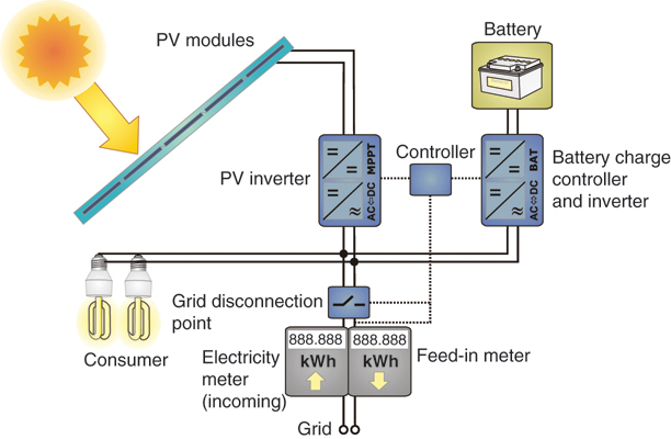
If a storage facility is combined with the PV system, significantly larger systems with higher degrees of self-sufficiency can be configured, which also benefit from high self-consumption levels. A wide range of battery systems are available for this purpose (Figure 5.15).
Figure 5.15 Grid-connected PV system with battery storage to increase the self-consumption level [Qua13].
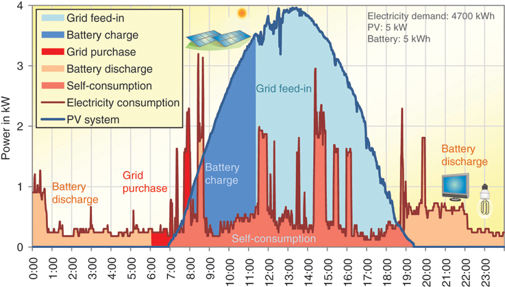
In battery systems, too, priority is given to using solar electricity directly on site. Any excess is used to charge a battery. Only when the battery is full does the system feed solar electricity into the grid. If the PV modules supply less electricity than is required on site, the battery initially covers the shortfall. Once the battery is empty, mains power is used to keep the system running (Figure 5.16). Modern battery systems can also relieve the public grid. For this purpose, they are not charged with the first surpluses from the solar system as shown in Figure 5.16. A forecast algorithm determines when the largest surpluses from the PV system will occur during the day and then stores them in the battery system instead of feeding them into the grid.
Figure 5.16 Power flows in a grid-connected PV battery system for a household in a detached house on a sunny Sunday in spring.
A battery system can also be designed so that it can be disconnected from the mains via a disconnection point in the event of a power failure. This means that it can continue to operate as a stand-alone system and, with the aid of the battery, ensure the power supply for a certain period of time. It then operates as an emergency power system and increases the security of the supply.
Lead-acid or lithium batteries can be used. Lead-acid batteries are familiar as starter batteries for cars. While lead-acid batteries are still frequently used in smaller stand-alone PV systems, lithium batteries have become established in grid-connected systems. Lithium batteries have a significantly longer service life. Lead-acid batteries can last for 5–10 years if used properly, lithium batteries for 20 years. They are also less sensitive to deep discharges. Battery rooms with lead-acid batteries must always be well ventilated, since the batteries can emit hydrogen, which can lead to the formation of oxyhydrogen gas.
Batteries have become standard components in many PV systems; their popularity has risen thanks to sharp cost reductions over recent years. Systems with hydrogen storage are an alternative to battery systems. Excess electricity is converted to hydrogen with the aid of an electrolysis unit and, if required, converted back to electricity via a fuel cell. Since these systems are significantly more expensive than battery systems, their market shares will remain low for the foreseeable future.
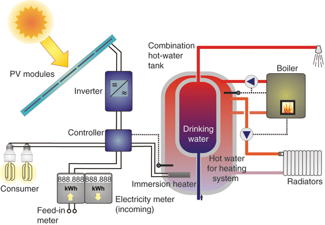
Another conceivable solution for increasing the share of self-consumption is coupling with an existing heating system (Figure 5.17). If a reasonably large heat store is available, an electric heating element can be retrofitted comparatively inexpensively. In principle, a more efficient heat pump can also be used instead of the heating element. However, since heat pumps are considerably more expensive, this significantly increases the capital costs and usually makes such a system economically unattractive, despite their greater efficiency. However, if a heat pump happens to be already available, then coupling with the PV system is essentially a ‘no-brainer’.
Figure 5.17 Coupling of a PV system with a conventional heating system becomes interesting when the feed-in tariff falls below the fuel costs.
Source: [Qua13].
Solar surpluses can then be used to heat the storage tank and thus save fuel in the heating system. In this way, the PV system can cover a larger part of the hot water demand and also supplement space heating in the spring and autumn. However, even with such a system, the majority of the heating demand is still covered by the conventional heating system and not by the PV system. It only makes economic sense to use the surplus solar energy when the tariff for the solar electricity fed into the grid falls below the fuel prices for heating.
5.4 Planning and Design
5.4.1 Designing Stand-Alone Systems
The design of stand-alone PV systems is fundamentally different from grid-connected systems. They cannot rely on the public electricity grid if there is no sun. Instead these systems use sufficiently large batteries to avoid any power failures. However, a battery should essentially only be used to bridge a small number of challenging days. Therefore, PV modules have to deliver as high a yield as possible during the months with the least sunshine. The recommendation for reliable operation in winter is to place PV modules at a steeper angle than is necessary with grid-connected systems, which are angled for optimum operation all year round. In Europe and North America, a tilt of around 60°–70° towards the south provides optimal solar yield in the month of December. The closer one gets to the equator, the less marked are the differences between summer and winter. In these parts of the world a shallower installation is sufficient for winter operation. In Cairo, for example, the optimum angle is around 50°. In Nairobi, however, an almost horizontal installation is recommended (Table 5.3).
Table 5.3Monthly and yearly totals of solar radiation in kWh/m2 for different locations and orientations
The aim of a stand-alone system is not to achieve the highest possible yield with a solar system, but to supply certain consumer loads reliably. Therefore, the system design should be based on the month with the poorest supply. In Germany, this is December. Furthermore, a solar system should have a safety margin of at least 50%. As with grid-connected systems, the performance ratio (PR) takes losses into account.
Required PV Module Output for Stand-Alone Systems
The required MPP output PMPP of the PV modules can be calculated approximately from the solar irradiation Hsolar,m in the worst month in kWh/m2, the electricity demand Edemand,m in the same month, a safety margin fS of at least 50% and the performance ratio PR (0.7 on average):
The battery should be dimensioned in such way that it is usually only half discharged and can meet the total electricity demand for a number of ‘reserve days’. In Central Europe up to five reserve days dR are enough to ensure reliable operation in the winter; in countries that get more sun two to three reserve days would be sufficient. If snow-covered PV modules are expected to be unable to supply electricity for a longer period of time in the winter, even more reserve days will be necessary. The required battery capacity is calculated on the basis of the battery voltage Vbat (e.g. 12 V):
For example, a PV system should be capable of operating an 11 W low-energy light bulb in a summerhouse for three hours every day in the winter. The monthly electricity demand for one month is then Edemand,m = 31 × 11 W × 3 h = 1023 Wh. With a safety margin of 50% = 0.5 and a performance ratio of 0.7, a module in Berlin orientated towards the south and tilted 60° then has a required MPP power of
With five reserve days and a battery voltage of 12 V, the battery capacity is
5.4.2 Designing Grid-Connected Systems
The first thing to do when planning a solar system is to check whether a system can actually be installed. From the perspective of planning and building laws and regulations, solar systems are structural components – even if they are simply screwed to the roof of a house. The authority responsible for local building regulations determines whether approval is necessary, and, if so, what type of approval. In most cases PV systems do not need approval from the local authority unless they are erected on a greenfield site. Complications arise when the sites for such systems are subject to architectural conservation laws. A permit from the relevant authority is required if a solar system is to be installed on or near a protected building. In addition to obtaining planning permission, it is always a good idea to consult the building regulations and the development plans of the local authority. These plans will include any conditions that the local authority has stipulated for the construction of PV systems.
If there are no legal obstacles, the planning phase can start. If a PV system is to be installed on the roof of a house, you must first determine which parts of the roof can be used for a solar thermal system (see Chapter 6). As PV systems are sensitive to shade, it is recommended that the part of the roof used to generate solar power is shade-free. The installation should not be placed near chimneys, aerials, and other roof structures.
Available PV Capacity
Once the type of solar module has been selected, an approximate calculation of the available PV capacity can be made, based on the remaining roof area A and the efficiency (see Table 5.1):
The available capacity on a useable area of 27.8 m2 with a module efficiency of 18% (0.18) is
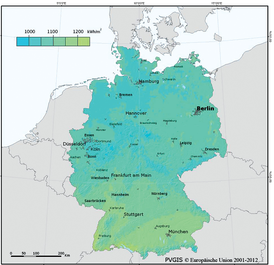
The annual system yield can be calculated based on this capacity. We must first determine the available solar energy. The map in Figure 5.18 shows the annual total solar radiation in Europe based on averages over many years. The radiation data for the USA can be found at http://www.nrel.gov/rredc. Fluctuations of over 10% in solar availability are possible between the individual years given. Since the 1980s, annual irradiation in Germany has increased by 5–10% due to a decrease in air pollution. Therefore, only relatively new radiation data should be used for the system design.
Figure 5.18 Mean annual total solar radiation energy in Germany in kWh/m2 between 1998 and 2011.
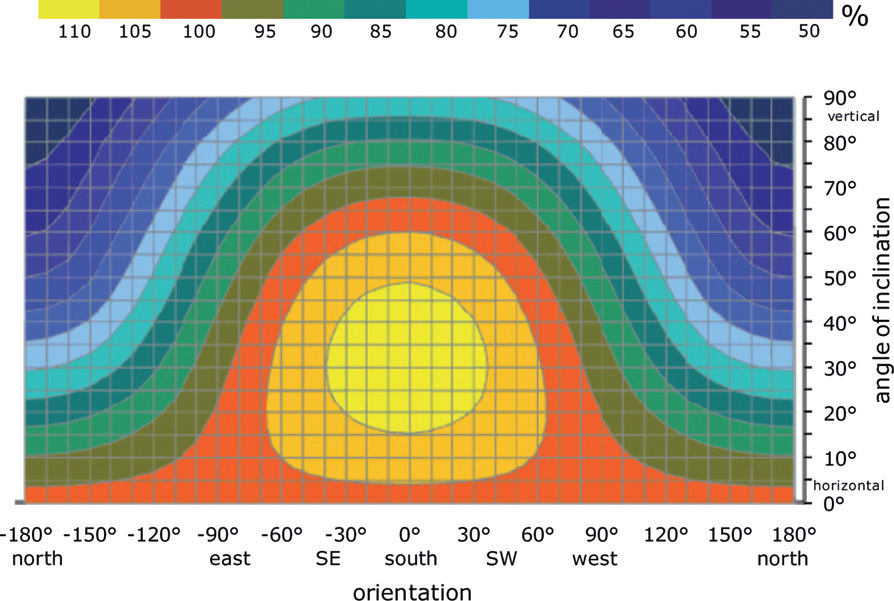
However, the values only apply to the horizontal orientation of a system. If a system is mounted on a sloping roof, the roof determines the orientation of the system. In Europe and North America, the roof should ideally be tilted around 35° to the south. With an optimal orientation towards the sun the supply of solar radiation increases by around 10%. However, good radiation values are still achievable even if the orientation is less favourable. Figure 5.19 shows the tilt gains and losses for all possible orientations for Berlin. These values can also be applied to other locations in central Europe.
Figure 5.19 Change in annual solar radiation in Berlin depending on orientation and tilt angle of PV systems.
If a PV system is to be installed on a roof or a greenfield site, the PV modules can be orientated optimally 35° towards the south. If the solar modules are set up in several rows one behind the other, they will shade each other as the sun goes down. A distance at least twice the module height should therefore be maintained between the module rows. This means that only around one-third of the area can be used. The loss due to shade then usually amounts to less than 5%.
The proportion of solar radiation that PV modules convert into electric energy depends on the quality of the system. Solar modules rarely achieve the rated power indicated. Dust, bird droppings, increases in air temperature, line losses, reflection, inverter losses, and other factors reduce performance. The relationship between real efficiency and rated efficiency is called the performance ratio (PR). Table 5.4 lists the criteria for performance ratio values for grid-connected PV systems.
Table 5.4Performance ratio of grid-connected PV systems
Performance ratio PR
Description
0.85
Top-quality system, very good ventilation, no shade, minimal pollution
0.8
Very good system, good ventilation, no shade
0.75
Average system
0.7
Average system with some losses due to shade or poor ventilation
0.6
Poor system with significant losses due to shade, pollution, or system failures
0.5
Very poor system with large areas of shade or defects
Electrical Energy Yield of Grid-Connected PV Systems
A rough calculation of the quantity of energy fed in annually by a grid-connected PV system can be made on the basis of the annual solar radiation Hsolar in kWh/(m2 a) from Figure 5.18, the losses or gains due to orientation and tilt angle ftilt (Figure 5.19), the rated or MPP power PMPP of the PV modules in kWp and the performance ratio
PR (cf. Table 5.4):
The yield of an unshaded PV system in Berlin with a tilt of 20° and an MPP output of 5 kWp is calculated here as an example. The annual solar radiation according to Figure 5.18 is around 1075 kWh (m2 a)−1. According to Figure 5.19, the tilt gains are ftilt = 110% = 1.1 based on a 20° south–south-west orientation. Based on the performance ratio of an average system PR = 0.8, the annual solar electricity yield is:
This corresponds to approximately the consumption of an average German single-family house. Therefore, as a yearly average about 30 m2 of roof area is needed for a household to cover its total electricity requirements using a solar system. The specific yield related to 1 kWp is often given for a system. In the example above, the total is 946 kWh (kWp a)−1.
The rough calculation of yield described here naturally incorporates certain inaccuracies. However, the order of magnitude of the system yield is correct. It can be used in the following section to examine the economic viability. Internet tools and computer programs are available to conduct a more precise analysis (see web addresses below). Professional firms also offer to carry out calculations of this type. In any case, if a large system is to be installed, it is advisable to get an expert to produce an appraisal on yield to avoid unpleasant surprises later on. Banks also often require a copy of the relevant appraisal.
It is not necessary for a grid-connected system to be large enough to cover the total electricity demand of a household. In the past, the size of the PV system was usually determined by the roof area. Quite often, the system capacity significantly exceeded the self-consumption level. In the future, systems that are optimized for self-consumption will become the norm. Large systems with a high degree of self-sufficiency not only promise increased independence from the energy supplier and its constantly rising electricity prices; but also make an important contribution to climate protection when they are installed in their millions.
5.4.3 Planned Autonomy
In the past, no further calculations were undertaken at this point, since all the solar power was fed into the grid and remunerated. Further considerations were therefore unnecessary. Today, however, the aim is to achieve high self-consumption levels to ensure good economic efficiency. In other situations, the aim is to achieve high degrees of self-sufficiency. This means one first needs to determine which proportion of the solar electricity generated is consumed locally and which is fed into the grid. The self-consumption and self-sufficiency levels depend on various parameters. The main influencing factors are the amount of electricity consumed and the size of the PV system. If a battery is added, the battery capacity naturally also plays a role.
The electricity bill makes it easy to determine one's own electricity consumption. The time period when the electricity is consumed also plays a role. In a pensioner's household, where electric cooking takes place every day at noon, the self-consumption level is higher than in the case of two working people who are mainly at home in the evening and at weekends. Compared to the other factors already mentioned, however, the type of household plays a lesser role. Therefore, to keep things simple, this influence is not considered.
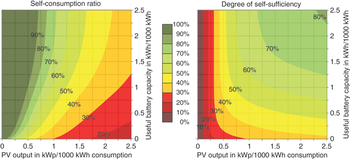
The self-consumption and self-sufficiency levels can be determined quite easily from Figure 5.20. For example, if a PV system with an output of 5 kWp is to be installed on a single-family house with an annual electricity consumption of 5000 kWh, the ratio of PV capacity in kWp to electricity consumption in 1000 kWh is 1.0. If no battery is provided, the usable battery capacity is zero. The self-consumption level is 30%. In other words, 70% of the solar electricity generated must be fed into the grid as excess. The self-sufficiency level is also 30%. This means that 70% of the local electricity consumption is still covered by an energy supplier via the grid. If a battery with a usable capacity of 5 kWh is added, the ratio of battery capacity to electricity consumption is also 1.0. This increases the self-consumption level to around 60% and the self-sufficiency level to over 50%.
Figure 5.20 Achievable self-consumption and self-sufficiency levels of PV self-consumption systems in single-family houses with battery storage [Wen13].
The self-consumption value determined in this way can then be used for the subsequent economic considerations. The self-consumption level reduces the consumption of electricity from the grid and reduces the electricity bill accordingly. Surpluses are fed into the grid based on the corresponding tariff. The cost-effectiveness of the PV system is based on mixed financing from saved electricity costs and feed-in revenues.
From Thinking About Having a PV System on the Roof to Getting a Quote
Determine the orientation and tilt angle of the roof. Is the roof suitable in terms of orientation and tilt angle? Recommendation: at least 95% according to Figure 5.19 on page
Establish shading conditions on the roof. Does my roof have any shade? Recommendation: take shaded areas into account during planning; also pay attention to chimneys, aerials, and lightning conductors. Identify available roof area with no shade.
Calculate installable MPP power for the PV system. Recommendation: Efficiency at least 16% in formula on page
Calculate possible annual electric energy yield. Use the formula on page or online tools.
Is the idea to increase the security of supply and the degree of self-sufficiency by using a battery?
Determine the self-consumption level according to Figure 5.20 on page.
Request quotes.
5.5 Economics
In some niche applications, PV has long been fully economically competitive. Small applications are often supplied with small batteries or button cells. Compared to household electricity prices of around 30 cents kWh−1 in Germany, for example, with PV the costs can quickly explode to several hundred euros per kWh. It takes around 280 AA-size high-quality alkaline manganese battery cells to store 1 kWh. However, no-one would ever consider buying 280 AA-size batteries to run a washing machine just once. Yet with small applications we often tend to be willing to pay whatever it costs to buy batteries. In many cases it is the infrequent use of these small applications that makes using electricity affordable in the first place. PV can compete with such high energy cost even under the most adverse conditions. Even with larger battery systems, PV is often an economical alternative. However, in order to effectively protect the climate, PV must do more than just domestic applications. This is only possible with grid-connected systems that replace conventional power plants.
5.5.1 What Does It Cost?
The minimum size for a grid-connected PV system is a PV module with about 0.3 kWp output. There is no upper limit; this depends only on the area and the amount of money available. Fortunately, the prices of PV systems are dropping so much that they are out of date even before they are printed. This makes it difficult for any published work to provide a current price guide. In 2005 the capital cost for a fully installed 5 kWp system without battery storage was around €30 000. In 2018, the figure was just €7000 excluding sales tax. The price of the PV module itself only constitutes part of the total system price. Around 50% of the capital cost is accounted for by the PV modules, while the rest is spent on inverters, mounting materials, the actual mounting, and planning. Prices for batteries have also fallen significantly in recent years. Further cost reductions are expected in the coming years.
Whereas the lion's share of the PV system cost is in the installation, the revenues then come through the electricity that is generated. The payment is usually per kWh. The operating costs of PV systems are comparatively low. Each year an estimated 2–5% of the capital cost is spent on running costs such as insurance, possible leasing, metre rental, and reserves for repairs. The modules can normally be used for 20–30 years. Repairs or replacements should be taken into account right from the start.
Another factor that has a major effect on generation costs is the return. Only very few idealists will invest their own capital in a PV system in the hope of at best receiving their invested capital back again over the lifetime of the system. The investment should yield a little more than a savings account in order to become attractive for larger groups of people. Even for this you need a certain amount of idealism, because the risk of a PV system is usually regarded as higher than that of a savings book. On the other hand, savings accounts are no longer what they used to be. Bank failures resulting in total loss of savings can no longer be ruled out.
A PV system, on the other hand, can be destroyed by a lightning strike or a storm. If the insurance does not pay for the damage, the investment is lost. Also, the yield may be less than predicted. There may be various reasons for this. The PV system could be the victim of poor planning, over the years a tree could grow so that it shuts out the sun, a flock of birds could regularly be using the module for target practice, or the solar radiation may be lower than during the previous 20 years due to volcanic eruptions. Ultimately, it is the operator of the PV system who is responsible for dealing with all these risks. A return of around 6% is therefore reasonable for an investment that is not driven by idealism. Conversely, self-consumption PV systems help to keep one's own electricity costs stable. The higher the price rises imposed by electricity suppliers, the more economical the PV system becomes.
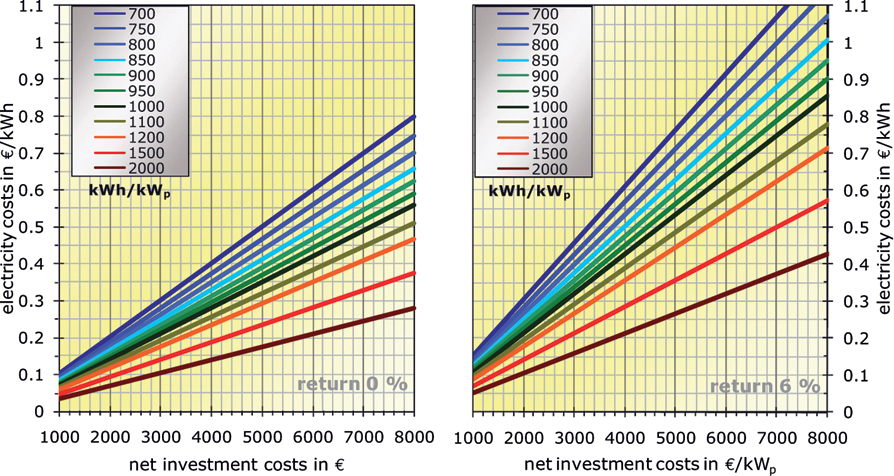
Figure 5.21 shows the resulting generating costs of a PV system without battery storage, depending on the net capital costs. The assumption made in the calculations is that 3.5% of the investment costs is for operating and maintenance costs each year and the economic lifetime of the system is 20 years. The different coloured lines represent the calculations for various specific yields. In Germany these are usually less than 1000 kWh kWp−1. For a return of 6% and net investment costs of €1500 per kW with a specific yield of 1000 kWh kWp−1, the resulting generation costs are 18.3 cents kWh−1. If the expected return is zero, 12.8 cents kWh−1 is sufficient. These costs must be generated on average from the electricity costs saved through self-consumption and the feed-in tariff.
Figure 5.21 Electricity generation costs as a function of net capital costs and specific yield for a return of 0% (left) and 6% (right).
5.5.2 Funding Programmes
While smaller stand-alone PV systems have long been competitive without any subsidies, larger grid-connected PV systems usually only pay for themselves if feed-in tariffs are available. Smaller systems can pay for themselves through the saved electricity costs, but here too an appropriate remuneration for feeding in surpluses is helpful. In Germany, the remuneration is determined by the Renewable Energy Sources Act (EEG). It prescribes a fixed price for every kilowatt hour that is fed into the public electricity supply grid by PV systems. The remuneration must be paid by the electricity supply company responsible, who may in turn pass on the additional costs incurred to all electricity customers. One aim is to make solar power competitive. Therefore, the law provides for a steady degression. The remuneration for new installations therefore decreases continuously. The remuneration is granted for a period of 20 years from the installation of the plant. The amount of remuneration decreases with the size of the system. Since 2016, PV systems with an output of more than 750 kW have had to successfully submit a tender application in order to receive funding.
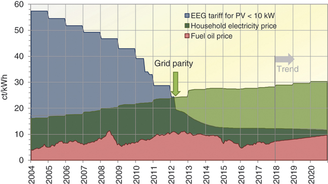
In 2012, grid parity was achieved. Since then, PV electricity has been cheaper than domestic electricity from the grid (Figure 5.22). This has fundamental effects on the PV market. While large PV systems were previously planned exclusively for grid feed-in and were not economical without feed-in tariffs, they are increasingly profitable due to electricity savings in self-consumption. In the meantime, even the difference between the remuneration for PV systems and the price of heating oil has become relatively small. In the foreseeable future, the feed-in tariff for solar power is expected to fall below the fuel costs for heating oil. This will certainly be the case for all PV systems for which the right to EEG compensation expires after 20 years. PV will then also become attractive as a supplement for heating systems.
Figure 5.22 Development of the EEG remuneration in Germany for small PV systems with outputs below 10 kW compared to the household electricity price and the fuel costs for oil heaters from 2004 to 2017 and trend from 2018 onwards.
The increased remuneration under the Renewable Energy Sources Act in Germany is expected to be phased out in the longer term. However, in order for PV to be completely competitive without subsidies, storage systems must become significantly cheaper. In order to achieve this, low-interest loans are envisaged for storage introduction programmes. In the past, low-interest loans were also available for the construction of PV systems in addition to the EEG remuneration, which are handled by the German Kreditanstalt für Wiederaufbau (KfW). Since the subsidy programmes are subject to rapid changes, it is advisable to enquire about the current conditions before installing a system (see web tip).
In Germany, a PV system for feeding into the grid can be operated privately or commercially. Losses can be written off from tax via a profit and loss account; profits must be taxed as income. This applies to both private and commercial operation. The purchase of the PV system may not be fully written off as a loss in the first year of operation, but it must have been fully paid off over 20 years.
The commercial operation of a PV system is particularly interesting in view of the Value Added Tax (VAT) refund. In principle, income from large PV systems is subject to VAT. For smaller plants with annual sales of less than €17 500, section 19 of the Value Added Tax Act applies, according to which the operator does not have to pay VAT and in return waives the reimbursement option. However, everyone can VAT-register, even if the threshold is not reached. In this case, the operation of the PV system must be reported to the tax office. As a rule, the tax office also expects proof of the intention to make a profit. Once you are VAT-registered, you have to add VAT on all goods and services sold, and then pay it to the tax office. However, the VAT is refunded for purchases. In the case of PV, VAT can then be refunded for the purchase of the system or repairs. This can quickly amount to a few hundred or thousand euros. However, the goods sold, i.e. the solar electricity, will then also be subject to VAT in the same way as the self-consumed solar electricity. VAT is added to the tariff set by the Renewable Energy Sources Act and thus does not reduce revenues.
However, the VAT reimbursement involves some bureaucratic effort. A VAT return is then due annually. For large plants with annual turnover tax revenue of more than €512 or with a combination of a small plant and a complicated tax official, a turnover tax return has to be submitted every month in advance. A wide range of computer programs are available to create tax returns and submit them electronically to the tax office.
Incidentally, there is no requirement to register small PV systems as a business, despite the voluntary VAT liability. This would, in any case, makes no sense, since business tax is only levied for profits over €24 500.
From the Quotation for a PV System for Grid Feed-in to the Installed System
The applicant should:
determine public subsidies and low-interest loans (see web tip);
check cost-effectiveness on the basis of the offer (see Figure 5.21);
register the planned installation with the energy supplier;
arrange for the system to be installed by a qualified company;
send the report completed by the electrician and technical system documents to the responsible energy supply company (ESC). ESC approves the plant and offers a feed-in contract in accordance with the EEG.
check the feed-in contract, amend it if necessary and sign it;
report the commercial operation of the PV system to the tax office;
have VAT paid via VAT return reimbursed as pre-tax deduction;
read the metre readings at the intervals agreed with the RU and pass them on to the ESC. Create invoice if appropriate;
if necessary, send monthly VAT return to the tax office; and
send annual profit and loss statement with income tax and VAT return to the tax office.
5.6 Ecology
There is a persistent rumour that it requires more energy to be used for the production of the silicon needed to make the solar cell than the cell itself can generate during its entire service life. Where this rumour came from is a mystery. It was probably invented by opponents of solar technology at a time when there were no detailed studies on the issue available.
It is true that the production of solar cells is relatively energy-intensive. Temperatures of well over 1000 °C are required for the production of silicon and subsequent purification. In contrast to conventional coal, gas, or nuclear power plants, however, no further energy input is required for the operation of PV systems. After commissioning, the solar system starts to return the energy required for its production. Various scientific studies in the 1990s have shown that in Germany it takes around two to three years for solar cells to generate the energy that was needed to produce them [Qua12], significantly less than two years in southern Europe. In the interim, thanks to the increased efficiencies and the reduced cell thicknesses, this time is likely to have decreased even further. With a service life of 20–30 years, a solar cell generates many times the energy that was required for its production.
Today, a 0.3 mm thick, 6-in. crystalline silicon solar cell weighs around 16 g. The energy consumption for the production of solar cells will decrease continuously, as attempts are made to drastically reduce the use of materials and thus also the costs. For example, in thin-film cells, the use of materials is already significantly lower. In the future, it can be expected that solar systems will recoup the energy needed to produce them within a few months.
Various chemicals, some of which are toxic, are used in the manufacture of solar cells, which is why, as with all chemical plants, strict care must be taken during production to ensure that no chemicals escape into the environment. However, in modern production plants with high environmental standards, this should be possible without any problems.
The finished solar system, on the other hand, is much less problematic. Nevertheless, it would be a pity to simply scrap old solar systems, as they contain valuable raw materials. The solar industry is therefore continuously improving its processes for recovering materials. Solar modules are broken down into their components, and the materials are separated by type.
5.7 PV Markets
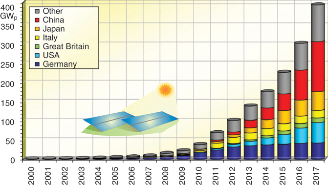
PV offers the most versatile application options of all the renewables. Their big advantage is the modular structure. Almost all desired generator sizes can be realized, starting from the milliwatt range for the power supply of pocket calculators and watches, up to the gigawatt range for the public power supply. While pocket calculators supplied with PV energy became widespread decades ago, large-scale systems that feed solar power into the public grid only became popular with the successful market launch programs in Japan and Germany. Government schemes in both countries boosted the production of PV modules and have contributed towards annual market growth rates between 20% and 80% since the early 1990s (Figure 5.23). In the meantime, other countries have also created attractive conditions for the construction of grid-connected PV systems. While in 1980 85% of solar modules were still manufactured in the USA, this proportion had shrunk to below 10% by 2005. Japan and Germany have lost the rank of the leading PV nations and were replaced by China from 2010. Today, China dominates the global PV market.
Figure 5.23 Development of total PV capacity installed worldwide.
In Germany, the spread of grid-connected PV systems began in the early 1990s with the so-called 1000 Roofs Programme. With the help of state schemes more than 2250 PV systems were erected, mainly by private households. When the programme was phased out, the use of PV began to stagnate. It was not until 2000 that fresh impetus was given through the introduction of the Renewable Energy Sources Act (EEG). Until 2012, the German PV market was the world's leading market and German solar companies were the world leaders.
In 2013, the German government significantly worsened the conditions for PV systems. The result was a radical market slump from 7.6 GW in 2012 to just 1.5 GW in 2016, resulting in a large number of German solar companies filing for insolvency. Around 80 000 jobs were lost in Germany.
At the end of 2017, well over one million PV systems, with an output of over 43 GW, were in operation in Germany. These systems fed 40 billion kilowatt hours of electric power into the grid, which was a 7% share of the overall electricity supply.
While from 2013 onwards Germany virtually put thumbscrews on the PV market, the PV expansion in China boomed at a breathtaking pace during the same period. In 2017 alone, China erected more PV systems than Germany had erected in the previous 30 years combined. China is unlikely to relinquish its dominant position in the coming years and is likely to remain the pacesetter in the field of PV.
5.8 Outlook and Development Potential
While just a few years ago PV was by far the most expensive way of generating electricity, today new PV systems can already outperform conventional power plants in many regions of the world. If the price decline continues, PV could become the most important type of electricity generation in the next 10–20 years.
Past experience has shown that major cost reductions are possible. Whereas the price of PV modules was still around 60 (inflation-adjusted) US dollars per watt in 1976, by 2012 it had already dropped to around $1 W−1 and by 2017 to 50 cents. This development over the years can be seen in a so-called learning curve (Figure 5.24). What is crucial for cutting costs is an increase in production. If production quantities rise, then costs will drop noticeably, due to the effects of streamlined production and also because of technical advances. During the past 30 years cost savings of around 20% have been achieved due to the total quantities of PV modules produced being doubled. There is nothing to indicate that this development will not continue.
Figure 5.24 Development of inflation-adjusted photovoltaic module prices as a function of the total volume of modules produced worldwide.
In purely mathematical terms, PV could even cover the entire global energy demand. This would only take a fraction of the surface of the Sahara Desert to accomplish. Even countries like Great Britain, Germany, and France would be able to cover all their electricity requirements through PV. On the other hand, from a technical perspective, it is not a good idea to rely solely on one technology for our energy supply of the future. PV systems work well in combination with other renewable energy systems, such as wind power, hydropower, and biomass systems. A sensible combination can increase supply security and avoid the construction of large storage facilities to ensure supply at night or in winter (Figure 5.25).
Figure 5.25 De-centralized PV systems can be set up by the electricity customers, directly, who thus become competitors to conventional energy suppliers and drive forward the energy transition.
PV has the potential to become the driving force behind the global energy transition. In contrast to larger power plants, PV can also be locally installed, directly with the end customer. The electricity customers themselves can thus become direct competitors to the energy suppliers and drive forward the transformation of the energy supply system. If this development is not deliberately slowed down, PV could supply more than half of the electricity generated worldwide by the middle of the century and thus make a decisive contribution to climate protection.