
Efficient recursive estimation of the Riemannian barycenter on the hypersphere and the special orthogonal group with applications
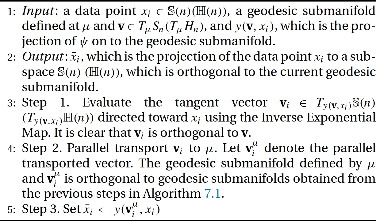
Rudrasis Chakraborty; Baba C. Vemuri University of Florida, CISE Department, Gainesville, FL, United States
Abstract
Finding the Riemannian barycenter (center of mass) or the Fréchet mean (FM) of manifold-valued data sets is a commonly encountered problem in a variety of fields of science and engineering, including, but not limited to, medical image computing, machine learning, and computer vision. For example, it is encountered in tasks such as atlas construction, clustering, principal geodesic analysis, and so on. Traditionally, algorithms for computing the FM of the manifold-valued data require that the entire data pool be available a priori and not incrementally. Thus, when encountered with new data, the FM needs to be recomputed over the entire pool, which can be computationally and storage inefficient. A computational and storage efficient alternative is to consider a recursive algorithm for computing the FM, which simply updates the previously computed FM when presented with a new data sample. In this chapter we present such an alternative called the inductive/incremental Fréchet mean estimator (iFME) for data residing on two well-known Riemannian manifolds, namely the hypersphere S(d)![]() and the special orthogonal group SO(d)
and the special orthogonal group SO(d)![]() . We prove the asymptotic convergence of iFME to the true FM of the underlying distribution from which the data samples were drawn. Further we present several experiments demonstrating the performance iFME on synthetic and real data sets.
. We prove the asymptotic convergence of iFME to the true FM of the underlying distribution from which the data samples were drawn. Further we present several experiments demonstrating the performance iFME on synthetic and real data sets.
Keywords
Fréchet Mean; Recursive Estimator; Hypersphere; SO(n); Gnomonic Projection; Weak Consistency
Acknowledgements
We thank Prof. David E. Vaillancourt and Dr. Edward Ofori for providing the diffusion MRI scans of movement disorder patients. We also thank Dr. Xavier Pennec and the anonymous reviewer for their invaluable comments in improving this manuscript. This research was in part supported by the NSF grants IIS-1525431 and IIS-1724174.
7.1 Introduction
Manifold-valued data have gained much importance in recent times due to their expressiveness and ready availability of machines with powerful CPUs and large storage. For example, these data arise as diffusion tensors (manifold of symmetric positive definite matrices) [1,2], linear subspaces (the Grassmann manifold) [3–8], column orthogonal matrices (the Stiefel manifold) [3,9–11], directional data and probability densities (the hypersphere) [12–15], and others. A useful method of analyzing manifold-valued data is to compute statistics on the underlying manifold. The most popular statistic is a summary of the data, that is, the Riemannian barycenter (Fréchet mean, FM) [16–18], Fréchet median [19,20], and so on.
FM computation on Riemannian manifolds has been an active area of research for the past few decades. Several researchers have addressed this problem, and we refer the reader to [21,18,22,23,19,24–27]. In most of these works, the authors relied on the standard gradient descent-based iterative computation of the FM, which suffers from two major drawbacks in an online computation setting: (1) for each new sample, it has to compute the new FM from scratch, and (2) it requires the entire input data to be stored to estimate the new FM. Instead, an incremental that is, a recursive technique can address this problem more efficiently with respect to time/space utility. In this age of massive and continuous streaming data, samples are often acquired incrementally. Hence, also from the applications perspective, the desired algorithm should be recursive/inductive to maximize computational efficiency and account for availability of data, requirements that are seldom addressed in more theoretically oriented fields.
Recently, several incremental mean estimators for manifold-valued data have been reported [28–31,5,32]. Sturm [29] presented an incremental mean, the so-called inductive mean, and proved its convergence to the true FM for all nonpositively curved (NPC) spaces. In [33] the authors showed several algorithms (including a recursive algorithm) for FM computation for data residing in CAT(0) spaces, which are NPC. They also demonstrated several applications of the same to computer vision and medical imaging. Further, in [31] an incremental FM computation algorithm along with its convergence and applications was presented for a population of symmetric positive definite (SPD) matrices. Recently, Lim [30] presented an inductive FM to estimate the weighted FM of SPD matrices. The convergence analysis in all of these works is applicable only to the samples belonging to NPC spaces, and hence their convergence analysis does not apply to the case of the manifolds with positive sectional curvature, which are our “objects” of interest in this chapter. Arnaudon et al. [34] present a stochastic gradient descent algorithm for barycenter computation of probability measures on Riemannian manifolds under some conditions. Their algorithm is quite general as it is applicable both to nonpositively and positively curved Riemannian manifolds.
In this work we present a novel incremental FM estimator (iFME) of a set of samples on two Riemannian manifolds of positive sectional curvature, that is, the hypersphere and the special orthogonal group. Data samples from either of these aforementioned manifolds are very commonly encountered in medical imaging, computer vision, and computer graphics. To mention a few, the directional data that are often encountered in image processing and computer vision are points on the unit 2-sphere S(2)![]() [12]. Further, 3×3
[12]. Further, 3×3![]() rotation matrices can be parameterized by unit quaternions, which can be represented by points on the projective space P(3)
rotation matrices can be parameterized by unit quaternions, which can be represented by points on the projective space P(3)![]() , i.e. couples of points and their antipodal point on the three-dimensional unit sphere S(3)
, i.e. couples of points and their antipodal point on the three-dimensional unit sphere S(3)![]() [15]. Also, any probability density function, for example, orientation distribution function (ODF) in diffusion magnetic resonance imaging (MRI) [14], can be represented as points on the positive quadrant of a unit Hilbert sphere [35,13].
[15]. Also, any probability density function, for example, orientation distribution function (ODF) in diffusion magnetic resonance imaging (MRI) [14], can be represented as points on the positive quadrant of a unit Hilbert sphere [35,13].
7.2 Riemannian geometry of the hypersphere
The hypersphere is a constant positive curvature Riemannian manifold that is commonly encountered in numerous application problems. Its geometry is well known, and here we will simply present (without derivations) the closed-form expressions for the Riemannian Exponential and Log maps as well as the geodesic between two points on it. Further, we also present the well-known square root parameterization of probability density functions (PDFs), which allows us to identify them with points on the unit Hilbert sphere. This will be needed in representing the probability density functions, namely, the ensemble average propagators (EAPs) derived from diffusion MRI, as points on the unit Hilbert sphere.
Without loss of generality we restrict the analysis to PDFs defined on the interval [0,T]![]() for simplicity: P={p:[0,T]→R|∀s,p(s)⩾0,∫T0p(s)ds=1}
for simplicity: P={p:[0,T]→R|∀s,p(s)⩾0,∫T0p(s)ds=1}![]() . In [26], the Fisher–Rao metric was introduced to study the Riemannian structure of a statistical manifold (the manifold of probability densities). For a PDF p∈P
. In [26], the Fisher–Rao metric was introduced to study the Riemannian structure of a statistical manifold (the manifold of probability densities). For a PDF p∈P![]() , the Fisher–Rao metric is defined as 〈v,w〉=∫T0v(s)w(s)p(s)ds
, the Fisher–Rao metric is defined as 〈v,w〉=∫T0v(s)w(s)p(s)ds![]() for v,w∈TpP
for v,w∈TpP![]() . The Fisher–Rao metric is invariant to reparameterizations of the functions. To facilitate easy computations when using Riemannian operations, the square root density representation ψ=√p
. The Fisher–Rao metric is invariant to reparameterizations of the functions. To facilitate easy computations when using Riemannian operations, the square root density representation ψ=√p![]() was used in [13], which was originally proposed in [36,37] and further developed from geometric statistics view point in [38]. The space of square root density functions is defined as Ψ={ψ:[0,T]→R|∀s,ψ(s)⩾0,∫T0ψ2(s)ds=1}
was used in [13], which was originally proposed in [36,37] and further developed from geometric statistics view point in [38]. The space of square root density functions is defined as Ψ={ψ:[0,T]→R|∀s,ψ(s)⩾0,∫T0ψ2(s)ds=1}![]() . As we can see, Ψ forms a convex subset of the unit sphere in a Hilbert space. Then, the Fisher–Rao metric can be written as 〈v,w〉=∫T0v(s)w(s)ds
. As we can see, Ψ forms a convex subset of the unit sphere in a Hilbert space. Then, the Fisher–Rao metric can be written as 〈v,w〉=∫T0v(s)w(s)ds![]() for tangent vectors v,w∈TψΨ
for tangent vectors v,w∈TψΨ![]() . Given any two functions ψi,ψj∈Ψ
. Given any two functions ψi,ψj∈Ψ![]() , the geodesic distance between these two points is given in closed form by d(ψi,ψj)=cos−1(〈ψi,ψj〉)
, the geodesic distance between these two points is given in closed form by d(ψi,ψj)=cos−1(〈ψi,ψj〉)![]() . The geodesic at ψ with a direction v∈TψΨ
. The geodesic at ψ with a direction v∈TψΨ![]() is defined as Γ(t)=cos(t)ψ+sin(t)v‖v‖
is defined as Γ(t)=cos(t)ψ+sin(t)v‖v‖![]() . The Riemannian exponential map can then be expressed by Expψ(v)=cos(‖v‖)ψ+sin(‖v‖)v‖v‖
. The Riemannian exponential map can then be expressed by Expψ(v)=cos(‖v‖)ψ+sin(‖v‖)v‖v‖![]() , where ‖v‖∈[0,π)
, where ‖v‖∈[0,π)![]() . The Riemannian inverse exponential map is then given by Logψi(ψj)=ucos−1(〈ψi,ψj〉)/√〈u,u〉
. The Riemannian inverse exponential map is then given by Logψi(ψj)=ucos−1(〈ψi,ψj〉)/√〈u,u〉![]() , where u=ψj−〈ψi,ψj〉ψi
, where u=ψj−〈ψi,ψj〉ψi![]() . Note that, for the rest of this chapter, we will assume that the data points are within a geodesic ball of radius less than the injectivity radius so that the Riemannian exponential is unique, and hence there always exists the corresponding inverse exponential map. We can define the geodesic between ψi
. Note that, for the rest of this chapter, we will assume that the data points are within a geodesic ball of radius less than the injectivity radius so that the Riemannian exponential is unique, and hence there always exists the corresponding inverse exponential map. We can define the geodesic between ψi![]() and ψj
and ψj![]() by Γψjψi(t)=cos(t)ψ+sin(t)v‖v‖
by Γψjψi(t)=cos(t)ψ+sin(t)v‖v‖![]() , where v=Logψi(ψj)
, where v=Logψi(ψj)![]() and t∈[0,1]
and t∈[0,1]![]() . We will use the term geodesic to denote the shortest geodesic between two points.
. We will use the term geodesic to denote the shortest geodesic between two points.
Using the geodesic distance provided previously, we can define the Fréchet mean (FM) [16,17] of a set of points on the hypersphere as the minimizer of the sum of squared geodesic distances (the so-called Fréchet functional). Let B(x,ρ)![]() be the geodesic ball centered at x with radius ρ, that is, B(x,ρ)={y∈S(k)|d(x,y)<ρ}
be the geodesic ball centered at x with radius ρ, that is, B(x,ρ)={y∈S(k)|d(x,y)<ρ}![]() . Authors in [39,18] showed that for any x∈Sk
. Authors in [39,18] showed that for any x∈Sk![]() and for data samples in B(x,π2)
and for data samples in B(x,π2)![]() , the minimizer of the Fréchet functional exists and is unique. For the rest of this chapter, we will assume that this condition is satisfied for any given set of points {xi}⊂S(k)
, the minimizer of the Fréchet functional exists and is unique. For the rest of this chapter, we will assume that this condition is satisfied for any given set of points {xi}⊂S(k)![]() . For more details on Riemannian geometry of the sphere, we refer the reader to Chapter 2 of [40] and references therein.
. For more details on Riemannian geometry of the sphere, we refer the reader to Chapter 2 of [40] and references therein.
7.3 Weak consistency of iFME on the sphere
In this section we present a detailed proof of convergence of our recursive estimator on the S(k)![]() . The proposed method is similar in “spirit” to the incremental arithmetic mean update in the Euclidean space; given the old mean mn−1
. The proposed method is similar in “spirit” to the incremental arithmetic mean update in the Euclidean space; given the old mean mn−1![]() and the new sample point xn
and the new sample point xn![]() , we define the new mean mn
, we define the new mean mn![]() as the weighted mean of mn−1
as the weighted mean of mn−1![]() and xn
and xn![]() with the weights n−1n
with the weights n−1n![]() and 1n
and 1n![]() , respectively. From a geometric viewpoint, this corresponds to the choice of the point on the geodesic between mn−1
, respectively. From a geometric viewpoint, this corresponds to the choice of the point on the geodesic between mn−1![]() and xn
and xn![]() with the parameter t=1n
with the parameter t=1n![]() , that is, mn=Γxnmn−1(1/n)
, that is, mn=Γxnmn−1(1/n)![]() .
.
Formally, let x1,x2,⋯,xN![]() be a set of N samples on the hypersphere S(k)
be a set of N samples on the hypersphere S(k)![]() , all of which lie inside a geodesic ball of radius π2
, all of which lie inside a geodesic ball of radius π2![]() . The incremental FM estimator (denoted by iFME) mn
. The incremental FM estimator (denoted by iFME) mn![]() with the given nth sample point xn
with the given nth sample point xn![]() is defined by
is defined by
m1=x1,
mn=Γxnmn−1(1n),
where Γxnmn−1![]() is the shortest geodesic path from mn−1
is the shortest geodesic path from mn−1![]() to xn
to xn![]() (∈Sk
(∈Sk![]() ), and 1n
), and 1n![]() is the weight assigned to the new sample point (in this case the nth sample), which is henceforth called the Euclidean weight. In the rest of this section we will show that if the number of given samples N tends to infinity, then the iFME estimates will converge to the expectation of the distribution from which the samples are drawn. Note that the geometric construction steps in the proof given further are not needed to compute the iFME; these steps are only needed to prove the weak consistency of iFME.
is the weight assigned to the new sample point (in this case the nth sample), which is henceforth called the Euclidean weight. In the rest of this section we will show that if the number of given samples N tends to infinity, then the iFME estimates will converge to the expectation of the distribution from which the samples are drawn. Note that the geometric construction steps in the proof given further are not needed to compute the iFME; these steps are only needed to prove the weak consistency of iFME.
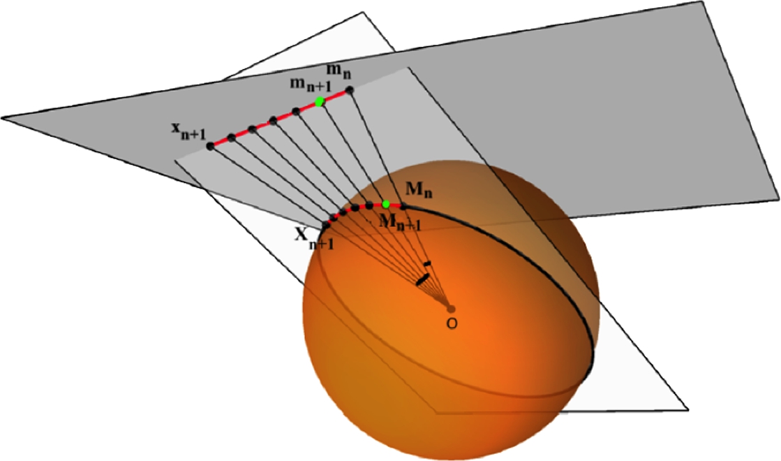
Our proof is based on the idea of projecting the samples xi![]() on the sphere to the tangent plane using the gnomonic projection [15] and performing the convergence analysis on the projected samples ˜xi
on the sphere to the tangent plane using the gnomonic projection [15] and performing the convergence analysis on the projected samples ˜xi![]() in this linear space, instead of performing the analysis on the hypersphere. We take advantage of the fact that the geodesic curve between any pair of points on the hemisphere is projected to a straight line in the tangent space at the anchor point (in this case, without loss of generality, assumed to be the north pole) via the gnomonic projection. A figure depicting the gnomonic projection is shown in Fig. 7.1. Despite the simplifications used in the statistical analysis of the iFME estimates on the hypersphere using the gnomonic projection, there is one important obstacle that must be considered. Without loss of generality, suppose the true FM of the input samples {xi}
in this linear space, instead of performing the analysis on the hypersphere. We take advantage of the fact that the geodesic curve between any pair of points on the hemisphere is projected to a straight line in the tangent space at the anchor point (in this case, without loss of generality, assumed to be the north pole) via the gnomonic projection. A figure depicting the gnomonic projection is shown in Fig. 7.1. Despite the simplifications used in the statistical analysis of the iFME estimates on the hypersphere using the gnomonic projection, there is one important obstacle that must be considered. Without loss of generality, suppose the true FM of the input samples {xi}![]() is the north pole. Then it can be shown through counter examples that:
is the north pole. Then it can be shown through counter examples that:
- • The use of Euclidean weights 1n
 to update the iFME estimates on S(k)
 does not necessarily correspond to the same weighting scheme between the old arithmetic mean and the new sample in the projection space, that is, the tangent space.
This fact can be illustrated using two sample points on a unit circle (S1![]() ), x1=(cos(π/6),sin(π/6))t
), x1=(cos(π/6),sin(π/6))t![]() and x2=(cos(π/3),sin(π/3))t
and x2=(cos(π/3),sin(π/3))t![]() , whose intrinsic mean is m=(cos(π/4),sin(π/4))t
, whose intrinsic mean is m=(cos(π/4),sin(π/4))t![]() . Then the midpoint of the gnomonic projections of x1
. Then the midpoint of the gnomonic projections of x1![]() and x2
and x2![]() , which are denoted by ˜x1
, which are denoted by ˜x1![]() and ˜x2
and ˜x2![]() , is ˆm=tan(π/3)+tan(π/6)2=1.1547≠tan(π/4)=˜m
, is ˆm=tan(π/3)+tan(π/6)2=1.1547≠tan(π/4)=˜m![]() (see Fig. 7.2).
(see Fig. 7.2).

For the rest of this section, without loss of generality, we assume that the FM of N given samples is located at the north pole. Since the gnomonic projection space is anchored at the north pole, this assumption leads to significant simplifications in our convergence analysis. However, a similar convergence proof can be developed for any arbitrary location of the FM, with the tangent (projection) space anchored at the location of this mean.
In what follows we prove that the use of Euclidean weights wn=1n![]() to update the incremental FM on the hypersphere corresponds to a set of weights in the projection space, denoted henceforth by tn
to update the incremental FM on the hypersphere corresponds to a set of weights in the projection space, denoted henceforth by tn![]() , for which the weighted incremental mean in the tangent plane converges to the true FM on the hypersphere, which in this case is the point of tangency.
, for which the weighted incremental mean in the tangent plane converges to the true FM on the hypersphere, which in this case is the point of tangency.
Theorem 7.1
Angle Bisector Theorem
[41] Let mn![]() and mn+1
and mn+1![]() denote the iFME estimates for n and n+1
denote the iFME estimates for n and n+1![]() given samples, respectively, and xn+1
given samples, respectively, and xn+1![]() denotes the (n+1)
denotes the (n+1)![]() th sample. Further, let ˜mn
th sample. Further, let ˜mn![]() , ˜mn+1
, ˜mn+1![]() , ˜xn+1
, ˜xn+1![]() be the corresponding points in the projection space. Then
be the corresponding points in the projection space. Then
tn=‖˜mn−˜mn+1‖‖˜xn+1−˜mn+1‖=‖˜mn‖‖˜xn+1‖×sin(d(mn,mn+1))sin(d(mn+1,xn+1)),

where d is the geodesic distance on the hypersphere.
Assumption
For the rest of this section, we will assume that the input samples {xi}![]() are within the geodesic ball B(x,ρ)
are within the geodesic ball B(x,ρ)![]() , where 0<ρ<π/2
, where 0<ρ<π/2![]() , for some x∈Sk
, for some x∈Sk![]() . This is needed for the uniqueness of the FM on the hypersphere (see [42]). □
. This is needed for the uniqueness of the FM on the hypersphere (see [42]). □
Then we bound tn![]() with respect to the radius ρ.
with respect to the radius ρ.
Lemma 7.1
Lower and Upper Bounds for tn![]()
With the same assumptions made as in Theorem 7.1, we have the following inequality:
cos(ρ)n⩽tn⩽1cos(ρ)3n.
Proof
Lower Bound To prove this lower bound for tn![]() , we find the lower bounds for each fraction on the right-hand side of Eq. (7.3). The first term reaches its minimum value if mn
, we find the lower bounds for each fraction on the right-hand side of Eq. (7.3). The first term reaches its minimum value if mn![]() is located at the north pole and xn+1
is located at the north pole and xn+1![]() is located on the boundary of the geodesic ball B(x,ρ)
is located on the boundary of the geodesic ball B(x,ρ)![]() . In this case, ‖˜mn‖=1
. In this case, ‖˜mn‖=1![]() and ‖˜xn+1‖=1cos(ρ)
and ‖˜xn+1‖=1cos(ρ)![]() . This implies that
. This implies that
‖˜mn‖‖˜xn+1‖⩾cos(ρ).

Next, note that based on the definition of iFME, this second fraction in (7.3) can be rewritten as sin(d(mn,mn+1))sin(d(mn+1,xn+1))=sin(d(mn,mn+1))sin(nd(mn,mn+1))=1Un−1(cos(d(mn,mn+1)))![]() , where Un−1
, where Un−1![]() (x) is the Chebyshev polynomial of the second kind [43]. For any x∈[−1,1]
(x) is the Chebyshev polynomial of the second kind [43]. For any x∈[−1,1]![]() , the maximum of Un−1(x)
, the maximum of Un−1(x)![]() is reached when x=1
is reached when x=1![]() , for which Un−1(1)=n
, for which Un−1(1)=n![]() . Therefore Un−1(x)⩽n
. Therefore Un−1(x)⩽n![]() and 1Un−1(x)⩾1n
and 1Un−1(x)⩾1n![]() . This implies that
. This implies that
sin(d(mn,mn+1))sin(nd(mn+1,mn+1))=1Un−1(cos(d(mn,mn+1)))⩾1n.

Note that as ρ tends to zero, cos(ρ)![]() converges to one, and this lower bound tends to 1n
converges to one, and this lower bound tends to 1n![]() , which is the case for the Euclidean space.
, which is the case for the Euclidean space.
Proof
Upper Bound First, the upper bound for the first term in (7.3) is reached when mn![]() is on the boundary of geodesic ball and xn+1
is on the boundary of geodesic ball and xn+1![]() is given at the north pole. Therefore
is given at the north pole. Therefore
‖˜mn‖‖˜xn+1‖⩽1cos(ρ).

Finding the upper bound for the sin term however is quite involved. Note that the maximum of the angle between mn![]() and xn+1
and xn+1![]() at the center of the S(k)
at the center of the S(k)![]() , denoted by α, is reached when mn
, denoted by α, is reached when mn![]() and xn+1
and xn+1![]() are both on the boundary of the geodesic ball, that is, α⩽2ρ
are both on the boundary of the geodesic ball, that is, α⩽2ρ![]() . Therefore ρ∈[0,π2)
. Therefore ρ∈[0,π2)![]() implies that α∈[0,π)
implies that α∈[0,π)![]() . Further we show in the next lemma that the following inequality holds for any α∈(0,π)
. Further we show in the next lemma that the following inequality holds for any α∈(0,π)![]() :
:
sin(nαn+1)sin(αn+1)⩾ncos2(α2)=ncos2(ρ).

Proof
Let f=sin(nθ)−ncos2(n+12θ)sin(θ)![]() , θ∈(0,α/(n+1))
, θ∈(0,α/(n+1))![]() , α∈(0,π)
, α∈(0,π)![]() , n⩾1
, n⩾1![]() , and fθ=ncos(nθ)+2ncos(n+12θ)sin(θ)sin(n+12θ)(n+12)−ncos2(n+12θ)cos(θ)
, and fθ=ncos(nθ)+2ncos(n+12θ)sin(θ)sin(n+12θ)(n+12)−ncos2(n+12θ)cos(θ)![]() . As θ∈(0,π/(n+1))
. As θ∈(0,π/(n+1))![]() , by solving the above equation we get θ=0
, by solving the above equation we get θ=0![]() . But fθθ|θ=0=0
. But fθθ|θ=0=0![]() . Hence we check fθθθ
. Hence we check fθθθ![]() : fθθθ|θ=0=−n3+1.5n(n+1)2+n>0
: fθθθ|θ=0=−n3+1.5n(n+1)2+n>0![]() , n⩾1
, n⩾1![]() . So, at θ=0
. So, at θ=0![]() , f has a minimum where θ∈(0,α/(n+1))
, f has a minimum where θ∈(0,α/(n+1))![]() and f|θ=0=0
and f|θ=0=0![]() . Thus f⩾0
. Thus f⩾0![]() as n⩾1
as n⩾1![]() . Since, for θ∈(0,α/(n+1))
. Since, for θ∈(0,α/(n+1))![]() , sin(θ)>0
, sin(θ)>0![]() , fsin(θ)⩾0
, fsin(θ)⩾0![]() fsin(θ)=sin(nθ)sin(θ)−ncos2(n+12θ)
fsin(θ)=sin(nθ)sin(θ)−ncos2(n+12θ)![]() . Hence sin(nθ)sin(θ)−ncos2(n+12θ)⩾0
. Hence sin(nθ)sin(θ)−ncos2(n+12θ)⩾0![]() . Then by substituting θ=α/(n+1)
. Then by substituting θ=α/(n+1)![]() we get sin(nαn+1)sin(αn+1)⩾ncos2(α2)
we get sin(nαn+1)sin(αn+1)⩾ncos2(α2)![]() . This completes the proof. □
. This completes the proof. □
Thus far we have shown analytical bounds for the sequence of weights tn![]() in the projection space corresponding to Euclidean weights on the sphere (Eq. (7.4)). We now prove the convergence of iFME estimates to the expectation of distribution from which the samples are drawn as the number of samples tends to infinity.
in the projection space corresponding to Euclidean weights on the sphere (Eq. (7.4)). We now prove the convergence of iFME estimates to the expectation of distribution from which the samples are drawn as the number of samples tends to infinity.
Theorem 7.2
Unbiasedness
Let (σ,ω)![]() denote a probability space with probability measure ω. A vector-valued random variable ˜x
denote a probability space with probability measure ω. A vector-valued random variable ˜x![]() is a measurable function on σ taking values in Rk
is a measurable function on σ taking values in Rk![]() , that is, ˜x
, that is, ˜x![]() : σ → Rk
: σ → Rk![]() . The distribution of ˜x
. The distribution of ˜x![]() is the push-forward probability measure dP(˜x)
is the push-forward probability measure dP(˜x)![]() =˜x⁎(σ)
=˜x⁎(σ)![]() on Rk
on Rk![]() . The expectation is defined by E[˜x]
. The expectation is defined by E[˜x]![]() =∫σ˜xdω
=∫σ˜xdω![]() . Let ˜x1,˜x2,…
. Let ˜x1,˜x2,…![]() be i.i.d. samples drawn from the distribution of ˜x
be i.i.d. samples drawn from the distribution of ˜x![]() . Also, let ˜mn
. Also, let ˜mn![]() be the incremental mean estimate corresponding to the nth given sample ˜xn
be the incremental mean estimate corresponding to the nth given sample ˜xn![]() , which is defined by: (i) ˜m1=˜x1
, which is defined by: (i) ˜m1=˜x1![]() , (ii) ˜mn=tn˜xn+(1−tn)˜mn−1
, (ii) ˜mn=tn˜xn+(1−tn)˜mn−1![]() . Then, ˜mn
. Then, ˜mn![]() is an unbiased estimator of the expectation E[˜x]
is an unbiased estimator of the expectation E[˜x]![]() .
.
Proof
For n=2![]() , ˜m2=t2˜x2+(1−t2)˜x1
, ˜m2=t2˜x2+(1−t2)˜x1![]() , and hence E[˜m2]=t2E[˜x]+(1−t2)E[˜x]=E[˜x]
, and hence E[˜m2]=t2E[˜x]+(1−t2)E[˜x]=E[˜x]![]() . By induction hypothesis we have E[˜mn−1]=E[˜x]
. By induction hypothesis we have E[˜mn−1]=E[˜x]![]() . Then E[˜mn]=tnE[˜x]+(1−tn)E[˜x]=E[˜x]
. Then E[˜mn]=tnE[˜x]+(1−tn)E[˜x]=E[˜x]![]() , hence the result. □
, hence the result. □
Theorem 7.3
Weak Consistency
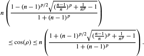
Let Var[˜mn]![]() denote the variance of the nth incremental mean estimate (defined in Theorem 7.2) with cos(ρ)n⩽tn⩽1cos(ρ)3n
denote the variance of the nth incremental mean estimate (defined in Theorem 7.2) with cos(ρ)n⩽tn⩽1cos(ρ)3n![]() for ϕ∈[0,π/2)
for ϕ∈[0,π/2)![]() . Then there exists p∈(0,1]
. Then there exists p∈(0,1]![]() such that Var[˜mn]Var[˜x]⩽(npcos6(ρ))−1
such that Var[˜mn]Var[˜x]⩽(npcos6(ρ))−1![]() .
.
First note that Var[˜mn]=t2nVar[˜x]+(1−tn)2Var[˜mn−1]![]() . Since, 0⩽tn⩽1
. Since, 0⩽tn⩽1![]() , we can see that Var[˜mn]⩽Var[˜x]
, we can see that Var[˜mn]⩽Var[˜x]![]() for all n. Besides, for each n, the maximum of the right-hand side is achieved when tn
for all n. Besides, for each n, the maximum of the right-hand side is achieved when tn![]() attains either its minimum or maximum value. Therefore we need to prove the theorem for the following two values of tn
attains either its minimum or maximum value. Therefore we need to prove the theorem for the following two values of tn![]() : (i) tn=cos(ρ)n
: (i) tn=cos(ρ)n![]() and (ii) tn=1ncos3(ρ)
and (ii) tn=1ncos3(ρ)![]() . These two cases will be proved in Lemmas 7.3 and 7.4, respectively.
. These two cases will be proved in Lemmas 7.3 and 7.4, respectively.
Lemma 7.3
Suppose the same assumptions as in Theorem 7.2 are made. Further, let tn=1ncos3(ρ)![]() for all n and all ρ∈[0,π/2)
for all n and all ρ∈[0,π/2)![]() . Then Var[˜mn]Var[˜x]⩽(ncos6(ρ))−1
. Then Var[˜mn]Var[˜x]⩽(ncos6(ρ))−1![]() .
.
Proof
For n=1![]() , Var[˜m1]=Var[˜x]
, Var[˜m1]=Var[˜x]![]() , which yields the result, since cos(ρ)⩽1
, which yields the result, since cos(ρ)⩽1![]() . Now assume by induction that Var[˜mn−1]Var[˜x]⩽(n−1)×cos6(ρ))−1
. Now assume by induction that Var[˜mn−1]Var[˜x]⩽(n−1)×cos6(ρ))−1![]() . Then
. Then
Var[˜mn]Var[˜x]=t2n+(1−tn)2Var[˜mn−1]Var[˜x]⩽t2n+(1−tn)21(n−1)cos6(ρ)⩽1cos6(ρ)n2+(1−1cos3(ρ)n)2×1(n−1)cos6(ρ)⩽1cos6(ρ)n2+(1−1n)2×1(n−1)cos6(ρ)=1cos6(ρ)n2+n−1n2cos6(ρ)=1ncos6(ρ).
□
Lemma 7.4
Suppose the same assumptions as in Theorem 7.2. Further, let tn=cos(ρ)n![]() for all n and all ϕ∈[0,π/2)
for all n and all ϕ∈[0,π/2)![]() . Then Var[˜mn]Var[˜x]⩽n−p
. Then Var[˜mn]Var[˜x]⩽n−p![]() for some 0<p⩽1
for some 0<p⩽1![]() .
.
Proof
For n=1![]() , Var[˜mn]=Var[˜x]
, Var[˜mn]=Var[˜x]![]() , which yields the result, since cos(ρ)⩽1
, which yields the result, since cos(ρ)⩽1![]() . Now assume by induction that Var[˜mn−1]Var[˜x]⩽(n−1)−p
. Now assume by induction that Var[˜mn−1]Var[˜x]⩽(n−1)−p![]() . Then
. Then
Var[˜mn]Var[˜x]=t2n+(1−tn)2Var[˜mn−1]Var[˜x]⩽t2n+(1−tn)21(n−1)p⩽cos2(ρ)n2+(n−cos(ρ))2n2×1(n−1)p=(n−1)pcos2(ρ)+cos2(ρ)−2ncos(ρ)+n2n2(n−1)p.

Now it suffices to show that the numerator of this expression is not greater than n2−p(n−1)p![]() . In other words,
. In other words,
(n−1)pcos2(ρ)+cos2(ρ)−2ncos(ρ)+n2−n2−p(n−1)p⩽0.
This quadratic function in cos(ρ)![]() is less than zero when
is less than zero when
n(1−(n−1)p/2√(n−1n)p+1np−11+(n−1)p)⩽cos(ρ)⩽n(1+(n−1)p/2√(n−1n)p+1np−11+(n−1)p).
The inequality on the right is satisfied for all values of the cos function. Besides, it is easy to see that the function on the left-hand side is increasing w.r.t. n>1![]() and hence attains its minimum when n=2
and hence attains its minimum when n=2![]() . This implies that
. This implies that
1−√21−p−1⩽cos(ρ)⇒ρ⩽cos−1(1−√21−p−1)⇒0<p⩽1−log2[(1−cos(ρ))2+1].

Note that p>0![]() for all ρ<π/2
for all ρ<π/2![]() . □
. □
Proof
Convergence Equipped with the previous two results, it is easy to see that for all ρ∈[0,π/2)![]() , there exists p satisfying 0<p⩽1
, there exists p satisfying 0<p⩽1![]() such that
such that
- – If tn=cos(ρ)n
 , then Var[˜mn]Var[˜x]⩽1np⩽1npcos6(ρ)
 , because cos(ρ)⩽1
 .
. - – If tn=1ncos3(ρ)
 , then Var[˜mn]Var[˜x]⩽1ncos6(ρ)⩽1npcos6(ρ)
 , because p⩽1
 .
.
These two pieces together complete the proof of convergence. □
The inequality in Theorem 7.3 implies that as n→∞![]() , for any ρ∈[0,π/2)
, for any ρ∈[0,π/2)![]() , the variance of iFME estimates in the projection space tends to zero. Besides, when ρ approaches π/2
, the variance of iFME estimates in the projection space tends to zero. Besides, when ρ approaches π/2![]() , the corresponding power of n and cos(ρ)
, the corresponding power of n and cos(ρ)![]() become very small, hence the rate of convergence gets slower. Note that instead of the weighting scheme used here (i.e., in the spirit of incremental mean in Euclidean space), we can choose a different weighting scheme that is intrinsic to the manifold (i.e., as a function of curvature) to speed up the convergence rate.
become very small, hence the rate of convergence gets slower. Note that instead of the weighting scheme used here (i.e., in the spirit of incremental mean in Euclidean space), we can choose a different weighting scheme that is intrinsic to the manifold (i.e., as a function of curvature) to speed up the convergence rate.
Now we will show that our proposed recursive FM estimator has a linear convergence rate.
Theorem 7.4
Convergence rate
Let x1,…,xN![]() be the samples on S(k)
be the samples on S(k)![]() drawn from any distribution. Then algorithm (7.2) has a linear convergence rate.
drawn from any distribution. Then algorithm (7.2) has a linear convergence rate.
Proof
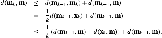
Let x1,…,xN![]() be the samples drawn from a distribution Sk
be the samples drawn from a distribution Sk![]() . Let m be the FM of {xi}
. Let m be the FM of {xi}![]() . Then, using the triangle inequality, we have
. Then, using the triangle inequality, we have
d(mk,m)⩽d(mk−1,mk)+d(mk−1,m)=1kd(mk−1,xk)+d(mk−1,m)⩽1k(d(mk−1,m)+d(xk,m))+d(mk−1,m).
Hence
d(mk,m)d(mk−1,m)⩽(1+1k+d(xk,m)kd(mk−1,m)).

Now, since d(mk−1,m)![]() and d(xk,m)
and d(xk,m)![]() are finite as {xi}
are finite as {xi}![]() are within a geodesic ball of radius <π/2
are within a geodesic ball of radius <π/2![]() , as k→∞
, as k→∞![]() , d(mk,m)d(mk−1,m)⩽1
, d(mk,m)d(mk−1,m)⩽1![]() . But the equality holds only if m lies on the geodesic between mk−1
. But the equality holds only if m lies on the geodesic between mk−1![]() and xk
and xk![]() . Let l<∞
. Let l<∞![]() , and let m lie on the geodesic between mk−1
, and let m lie on the geodesic between mk−1![]() and xk
and xk![]() for some k>l
for some k>l![]() . As m is fixed, using induction, we can easily show that m cannot lie on the same geodesic for all k>l
. As m is fixed, using induction, we can easily show that m cannot lie on the same geodesic for all k>l![]() . Hence d(mk,m)d(mk−1,m)<1
. Hence d(mk,m)d(mk−1,m)<1![]() , and the convergence rate is linear. □
, and the convergence rate is linear. □
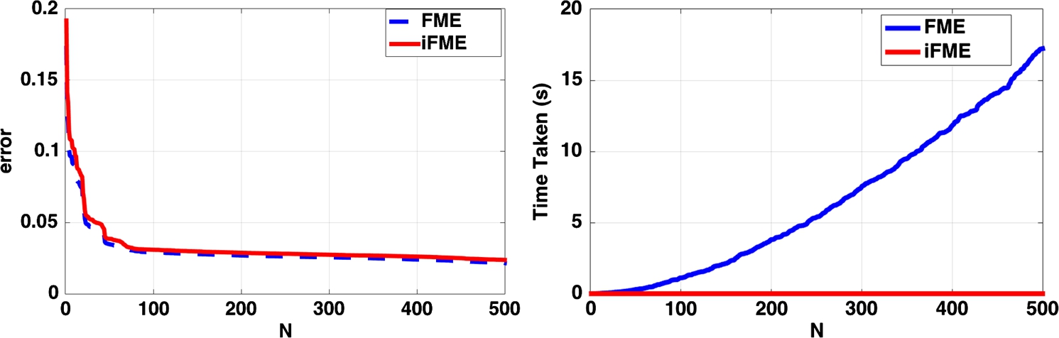
7.4 Experimental results
We now evaluate the effectiveness of the iFME algorithm, compared to the nonincremental counterpart FME, for computing the FM of a finite set of samples on the sphere (northern hemisphere not including the equator). For FME, we used a gradient descent technique to minimize the sum of squared geodesic distances cost function. We report the results for samples drawn from a Log-Normal distribution (with mean at the north pole and the variance set to 0.2) on the upper hemisphere. A set of random samples are drawn from the distribution and incrementally input to both iFME and FME algorithms. The computation time needed for each method to compute the sample FM and the error were recorded for each new sample incrementally introduced. In all the experiments the computation time is reported for execution on a 3.3 GHz desktop with a quadcore Intel i7 processor and 24 GB RAM. The error is defined by the geodesic distance between the estimated mean (using either iFME or FME) and the expectation of the input distribution. Because of the randomness in generating the samples, we repeated this experiment 100 times for each case, and the mean execution time and the error for each method are shown.
The performances of iFME and FME are evaluated with respect to the execution time and error and are illustrated in Fig. 7.3. From these plots we can clearly see that iFME performs almost equally good in terms of error/accuracy but takes comparatively very less execution time.
7.5 Application to the classification of movement disorders
In this section we use an exact-PGA (exact principal geodesic analysis) algorithm presented in [44], which is applicable to data residing on a hypersphere. We will call this the ePGA algorithm. We will also use the tangent PCA (tPCA) algorithm presented in [45] for diffusion tensor fields as a comparison. This algorithm consists of (1) computing the FM of the input data, (2) projecting each data point to the tangent space at the FM using the Riemannian log-map, (3) performing standard PCA in the tangent plane, and (4) projecting the result (principal vectors) back to the manifold using the Riemannian exponential map.
In the ePGA algorithm we will use iFME to compute the FM and make use of the parallel transport operation on the hypersphere. For completeness, we now present the ePGA algorithm from [44] and used here.
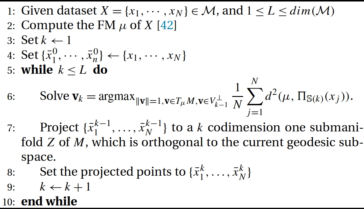
 .
.The projection algorithm/step in the above algorithm has an analytic expression for manifolds with constant sectional curvature, that is, for hypersphere and hyperbolic space. Here we will present the projection algorithm.
Note that the parallel transport operation on the hypersphere can be expressed in analytic form. The formula for parallel transporting u∈TnS(k)![]() from n to m is given by
from n to m is given by
w=Γn→m(p)=(p−v(vtp‖v‖2))+vtp‖v‖2(n(−sin(‖v‖)‖v‖)+vcos(‖v‖)),

where v=Lognm![]() . We refer the reader to [44] for details of the ePGA algorithm.
. We refer the reader to [44] for details of the ePGA algorithm.
The dataset for classification consists of high angular resolution diffusion image (HARDI) scans from (1) healthy controls, patients with (2) Parkinson's disease (PD), and (3) essential tremor (ET). We aim to automatically discriminate between these three classes using features derived from the HARDI data. This dataset consists of 25 controls, 24 PD, and 15 ET images. The HARDI data were acquired using a 3T Phillips MR scanner with the following parameters: TR=7748![]() ms, TE=86
ms, TE=86![]() ms, b-values: 0, 1000smm2
ms, b-values: 0, 1000smm2![]() , 64 gradient directions, and voxel size = 2×2×2mm3
, 64 gradient directions, and voxel size = 2×2×2mm3![]() .
.
Authors in [46] employed DTI-based analysis using scalar-valued features to address the problem of movement disorder classification. Later in [47] a PGA-based classification algorithm was proposed using Cauchy deformation tensors (computed from a nonrigid registration of patient scans to a HARDI control atlas), which are SPD matrices. In the next subsection we develop classification method based on (1) Ensemble Average Propagators (EAPs) derived from HARDI data within an ROI and (2) shapes of the ROI derived from the input population. Using a square root density parameterization [48], both features can be mapped to points on an unit Hilbert sphere, where the proposed iFME in conjunction with the ePGA method is applicable.
Classification results using the ensemble average propagator as features: To capture the full diffusional information, we chose to use the ensemble average propagator (EAP) at each voxel as our feature in the classification. We compute the EAPs using the method described in [49] and use the square root density parameterization of each EAP. This way the full diffusion information at each voxel is represented as a point on the unit Hilbert sphere.
We now present the classification algorithm, which is a combination of ePGA-based reduced representation and a nearest-neighbor classifier. The input to the ePGA algorithm are EAP features in this case. The input HARDI data are first rigidly aligned to the atlas computed from the control (normal) group, then EAPs are computed in a 3-D region of interest (ROI) in the midbrain. Finally, the EAP field extracted from each ROI image is identified with a point on the product manifold (the number of elements in the product is equal to the number of voxels in the ROI) of unit Hilbert spheres. This is in spirit similar to the case of the product manifold formalism in [45,47].
A set of 10 control, 10 PD, and 5 ET images are randomly picked as the test set, and the rest of the images are used for training. Also, classification is performed using ePGA, tPCA, and the standard PCA and is repeated 300 times to report the average accuracy. The results using EAP features are summarized in Table 7.2. It is evident that the accuracy of ePGA is better than that of the tPCA, whereas both methods are considerably more accurate than the standard PCA, as they account for the nonlinear geometry of the sphere.
Classification results using the shape features: In this section we evaluated the ePGA algorithm based on shape of the Substantia Nigra region in the given brain images for the task of movement disorder classification. We first collected random samples (point) on the boundary of each 3-D shape and applied the Schrödinger distance transform (SDT) technique in [50] to represent each shape as a point on the unit hypersphere. The size of the ROI for the 3-D shape of interest was set to 28×28×15![]() , and the resulting samples lie on an S11759
, and the resulting samples lie on an S11759![]() manifold. Then we used ePGA for classification. The results reported in Table 7.1 depict the accuracy gained in classification when using ePGA compared to tPCA. Evidently, ePGA yields a better classification accuracy.
manifold. Then we used ePGA for classification. The results reported in Table 7.1 depict the accuracy gained in classification when using ePGA compared to tPCA. Evidently, ePGA yields a better classification accuracy.
Table 7.1
Classification results from ePGA, tPCA, and PCA.
| Results using shape features | |||||||||
|---|---|---|---|---|---|---|---|---|---|
| Control vs. PD | Control vs. ET | PD vs. ET | |||||||
| ePGA | tPCA | PCA | ePGA | tPCA | PCA | ePGA | tPCA | PCA | |
| Accuracy | 94.5 | 93.0 | 67.3 | 91.4 | 90.1 | 75.7 | 88.1 | 87.6 | 64.6 |
| Sensitivity | 92.3 | 91.0 | 52.0 | 87.5 | 86.2 | 80.1 | 84.7 | 82.4 | 58.4 |
| Specificity | 96.8 | 95.0 | 82.7 | 96.3 | 94.1 | 71.3 | 94.2 | 92.8 | 70.8 |

Table 7.2
Classification results from ePGA, tPCA, and PCA.
| Results using EAP features | |||||||||
|---|---|---|---|---|---|---|---|---|---|
| Control vs. PD | Control vs. ET | PD vs. ET | |||||||
| ePGA | tPCA | PCA | ePGA | tPCA | PCA | ePGA | tPCA | PCA | |
| Accuracy | 93.7 | 93.5 | 59.8 | 92.8 | 91.3 | 70.2 | 92.4 | 90.9 | 66.0 |
| Sensitivity | 93.1 | 91.8 | 48.3 | 90.7 | 89.7 | 79.8 | 86.2 | 84.7 | 56.3 |
| Specificity | 96.9 | 95.2 | 71.3 | 93.1 | 92.9 | 60.6 | 98.7 | 97.1 | 75.7 |

7.6 Riemannian geometry of the special orthogonal group
The set of all n×n![]() orthogonal matrices is denoted by O(n)
orthogonal matrices is denoted by O(n)![]() , that is, O(n)={X∈Rn×n|XTX=In}
, that is, O(n)={X∈Rn×n|XTX=In}![]() . The set of orthogonal matrices with determinant 1, denoted by the special orthogonal group so(n)
. The set of orthogonal matrices with determinant 1, denoted by the special orthogonal group so(n)![]() , forms a compact subset of O(n)
, forms a compact subset of O(n)![]() . As so(n)
. As so(n)![]() is a compact Riemannian manifold, by the Hopf–Rinow theorem it is also a geodesically complete manifold [51]. Its geometry is well understood, and we recall a few relevant concepts here and refer the reader to [51] for details. The manifold so(n)
is a compact Riemannian manifold, by the Hopf–Rinow theorem it is also a geodesically complete manifold [51]. Its geometry is well understood, and we recall a few relevant concepts here and refer the reader to [51] for details. The manifold so(n)![]() has a Lie group structure, and the corresponding Lie algebra is defined as so(n)={W∈Rn×n|WT=−W}
has a Lie group structure, and the corresponding Lie algebra is defined as so(n)={W∈Rn×n|WT=−W}![]() . In other words, so(n)
. In other words, so(n)![]() (the set of Left invariant vector fields with associated Lie bracket) is the set of n×n
(the set of Left invariant vector fields with associated Lie bracket) is the set of n×n![]() antisymmetric matrices. The Lie bracket [,]
antisymmetric matrices. The Lie bracket [,]![]() , operator on so(n)
, operator on so(n)![]() , is defined as the commutator, that is, [U,V]=UV−VU
, is defined as the commutator, that is, [U,V]=UV−VU![]() for U,V∈so(n)
for U,V∈so(n)![]() . Now we can define a Riemannian metric on so(n)
. Now we can define a Riemannian metric on so(n)![]() as follows: 〈U,V〉X=trace(UTV)
as follows: 〈U,V〉X=trace(UTV)![]() for U,V∈TXso(n)
for U,V∈TXso(n)![]() , X∈so(n)
, X∈so(n)![]() . Note that it can be shown that this is a biinvariant Riemannian metric. Under this biinvariant metric, now we define the Riemannian exponential and inverse exponential maps as follows. Let X,Y∈so(n)
. Note that it can be shown that this is a biinvariant Riemannian metric. Under this biinvariant metric, now we define the Riemannian exponential and inverse exponential maps as follows. Let X,Y∈so(n)![]() , U∈TXso(n)
, U∈TXso(n)![]() . Then the Riemannian inverse exponential map is defined as
. Then the Riemannian inverse exponential map is defined as
LogX(Y)=Xlog(XTY),
and the Riemannian exponential map is defined as
ExpX(U)=Xexp(XTU),
where exp and log are the matrix exponential and logarithm, respectively. Due of the computational complexity of matrix exponential, we may instead choose to use the Riemannian retraction map as follows. Given W∈so(n)![]() , the Cayley map is a conformal mapping Cay:so(n)
, the Cayley map is a conformal mapping Cay:so(n)![]() →so(n)
→so(n)![]() defined by Cay(W)=(In+W)(In−W)−1
defined by Cay(W)=(In+W)(In−W)−1![]() . Using the Cayley map, we can define the Riemannian retraction map as, RetX
. Using the Cayley map, we can define the Riemannian retraction map as, RetX![]() :TXso(n)→so(n)
:TXso(n)→so(n)![]() by RetX(W)=Cay(W)X
by RetX(W)=Cay(W)X![]() . Using the Riemannian exponential (retraction) and inverse exponential map, we can define the geodesic on so(n)
. Using the Riemannian exponential (retraction) and inverse exponential map, we can define the geodesic on so(n)![]() as ΓYX(y)=Exp(tLogX(Y))
as ΓYX(y)=Exp(tLogX(Y))![]() .
.
7.7 Weak consistency of iFME on so(n)
In this section we present a detailed proof of convergence of our recursive estimator on so(n)![]() . Analogous to our FM estimator on S(k)
. Analogous to our FM estimator on S(k)![]() , we first define the FM estimator on so(n)
, we first define the FM estimator on so(n)![]() and then prove its consistency.
and then prove its consistency.
Formally, let X1,…,XN![]() be a set of N samples on so(n)
be a set of N samples on so(n)![]() , all of which lie inside a geodesic ball of an appropriate radius such that FM exists and is unique. The iFME estimate Mn
, all of which lie inside a geodesic ball of an appropriate radius such that FM exists and is unique. The iFME estimate Mn![]() of the FM with the nth given sample Xn
of the FM with the nth given sample Xn![]() is defined by
is defined by
M1=X1,
Mn=ΓXnMn−1(1n),
where ΓXnMn−1![]() is the shortest geodesic path from Mn−1
is the shortest geodesic path from Mn−1![]() to Xn
to Xn![]() (∈so(n)
(∈so(n)![]() ). In what follows we will show that as the number of given samples N tends to infinity, the iFME estimates will converge to the expectation of the distribution from which the samples are drawn.
). In what follows we will show that as the number of given samples N tends to infinity, the iFME estimates will converge to the expectation of the distribution from which the samples are drawn.
Theorem 7.5
Let X1,X2,…,XN![]() be i.i.d. samples drawn from a probability distribution on so(n)
be i.i.d. samples drawn from a probability distribution on so(n)![]() . Then the inductive FM estimator (iFME) MN
. Then the inductive FM estimator (iFME) MN![]() of these samples converges to M as N→∞
of these samples converges to M as N→∞![]() , where M is the expectation of the probability distribution.
, where M is the expectation of the probability distribution.
Proposition 7.1
Any arbitrary element of so(n)![]() can be written as the composition of planar rotations in the planes generated by the n standard orthogonal basis vectors of Rn
can be written as the composition of planar rotations in the planes generated by the n standard orthogonal basis vectors of Rn![]() .
.
Proof
Let X∈so(n)![]() . Observe that log(X)∈so(n)
. Observe that log(X)∈so(n)![]() . Further, log(X)
. Further, log(X)![]() is a skew-symmetric matrix. Let U=log(X)
is a skew-symmetric matrix. Let U=log(X)![]() . Then Uij
. Then Uij![]() is the angle of rotation in the plane formed by the basis vectors ei
is the angle of rotation in the plane formed by the basis vectors ei![]() and ej
and ej![]() for all i=1,…,n
for all i=1,…,n![]() and j=i+1,…,n
and j=i+1,…,n![]() . □
. □
By Proposition 7.1 we can express X as a product of n(n−1)/2![]() planar rotation matrices. Each planar rotation matrix can be mapped onto S(n−1)
planar rotation matrices. Each planar rotation matrix can be mapped onto S(n−1)![]() , hence there exists a mapping F:SO(n)
, hence there exists a mapping F:SO(n)![]() →S(n−1)×⋯×Sn−1︸n(n−1)/2 times
→S(n−1)×⋯×Sn−1︸n(n−1)/2 times![]() . Let us denote this product space of hyperspheres by O(n−1,n(n−1)2)
. Let us denote this product space of hyperspheres by O(n−1,n(n−1)2)![]() . Then F is a embedding of SO(n)
. Then F is a embedding of SO(n)![]() in O(n−1,n(n−1)2)
in O(n−1,n(n−1)2)![]() . Notice that as this product space has n(n−1)/2
. Notice that as this product space has n(n−1)/2![]() components, we will use two indices (i,j)
components, we will use two indices (i,j)![]() to denote a component. Hence, given X∈SO(n)
to denote a component. Hence, given X∈SO(n)![]() , the (i,j)
, the (i,j)![]() th component of F(X)
th component of F(X)![]() has ith and jth entries cos(θij)
has ith and jth entries cos(θij)![]() and sin(θij)
and sin(θij)![]() , respectively, and the rest of the n−2
, respectively, and the rest of the n−2![]() entries are zero. Here θij
entries are zero. Here θij![]() is the planar rotation angle in the plane spanned by ei
is the planar rotation angle in the plane spanned by ei![]() and ej
and ej![]() . The following propositions allow us to prove that SO(n)
. The following propositions allow us to prove that SO(n)![]() is a submanifold of O(n−1,n(n−1)2)
is a submanifold of O(n−1,n(n−1)2)![]() .
.
To do that, we will first use the Log-Euclidean metric on SO(n)![]() defined as follows: Given X,Y∈SO(n)
defined as follows: Given X,Y∈SO(n)![]() , the metric d(X,Y)=12‖log(X)−log(Y)‖F
, the metric d(X,Y)=12‖log(X)−log(Y)‖F![]() . Notice that this metric is adjoint invariant, as ‖Zlog(X)ZT−Zlog(Y)ZT‖F
. Notice that this metric is adjoint invariant, as ‖Zlog(X)ZT−Zlog(Y)ZT‖F![]() =‖log(X)−log(Y)‖F
=‖log(X)−log(Y)‖F![]() for some Z∈SO(n)
for some Z∈SO(n)![]() .
.
The following proposition shows that F is an isometric mapping using the product ℓ2![]() arc-length metric on O(n−1,n(n−1)2)
arc-length metric on O(n−1,n(n−1)2)![]() .
.
Proposition 7.2
F is an isometric mapping from SO(n)![]() to O(n−1,n(n−1)2)
to O(n−1,n(n−1)2)![]() .
.
Proof
Given X,Y∈SO(n)![]() , let F(X)ij
, let F(X)ij![]() and F(Y)ij
and F(Y)ij![]() be the (i,j)
be the (i,j)![]() th entries of F(X)
th entries of F(X)![]() and F(Y)
and F(Y)![]() , respectively. Let F(X)ij=(0⋯,0,cos(θXij),0,⋯,0,sin(θXij),0,⋯,0)t
, respectively. Let F(X)ij=(0⋯,0,cos(θXij),0,⋯,0,sin(θXij),0,⋯,0)t![]() and F(Y)ij=(0,…,0,cos(θYij),0,…,0,sin(θYij),0,…,0)t
and F(Y)ij=(0,…,0,cos(θYij),0,…,0,sin(θYij),0,…,0)t![]() . Then F(X)ij,F(Y)ij∈Sn−1
. Then F(X)ij,F(Y)ij∈Sn−1![]() , and hence d(F(X)ij,F(Y)ij)=|θXij−θYij|
, and hence d(F(X)ij,F(Y)ij)=|θXij−θYij|![]() . Thus the (i,j)
. Thus the (i,j)![]() th entry of log(X)−log(Y)
th entry of log(X)−log(Y)![]() is the signed distance d(F(X)ij,F(Y)ij)
is the signed distance d(F(X)ij,F(Y)ij)![]() . This concludes the proof. □
. This concludes the proof. □
It is easy to see that the ΓYX![]() from X to Y is given by
from X to Y is given by
ΓYX(t)=exp(log(X)+t(log(Y)−log(X))).
In the following propositions we will show that F maps ΓXY![]() to the (shortest) geodesic from F(X)
to the (shortest) geodesic from F(X)![]() to F(Y)
to F(Y)![]() for any X,Y∈SO(n)
for any X,Y∈SO(n)![]() .
.
Proposition 7.3
Proof
From spherical geometry we know that given x,y∈Sn−1![]() , the shortest geodesic is given by
, the shortest geodesic is given by
Γyx(t)=1sin(θ)(sin(tθ)x+sin((1−t)θ)y),

where θ=d(x,y)![]() . Now, given the hypothesis: θ=|θ2−θ1|
. Now, given the hypothesis: θ=|θ2−θ1|![]() , observe that, for t∈[0,1]
, observe that, for t∈[0,1]![]() , Γyx(t)
, Γyx(t)![]() is the unique point on Sn−1
is the unique point on Sn−1![]() such that d(Γyx(t),x)=t|θ2−θ1|
such that d(Γyx(t),x)=t|θ2−θ1|![]() and d(Γyx(t),y)=(1−t)|θ2−θ1|
and d(Γyx(t),y)=(1−t)|θ2−θ1|![]() . Substituting
. Substituting
Γyx(t)=((0,…,0,cos(tθ1+(1−t)θ2)),0,…,0,sin(tθ1+(1−t)θ2),0,…,0)t,
we conclude the proof. □
Theorem 7.6
SO(n)![]() is a geodesic submanifold of O(n−1,n(n−1)2)
is a geodesic submanifold of O(n−1,n(n−1)2)![]() .
.
Proof
Given X,Y∈SO(n)![]() and t∈[0,1]
and t∈[0,1]![]() , the shortest geodesic is given by ΓYX(t)=exp(log(X)+t(log(Y)−log(X)))
, the shortest geodesic is given by ΓYX(t)=exp(log(X)+t(log(Y)−log(X)))![]() . Now observe that
. Now observe that
F(X)ij=(0,…,0,cos(θ1),0,…,0,sin(θ1),0,…,0)t,
where θ1=log(X)ij![]() , and
, and
F(Y)ij=(0,…,0,cos(θ2),0,…,0,sin(θ2),0,…,0)t,
where θ2=log(Y)ij![]() . By Proposition 7.3,
. By Proposition 7.3,
log(F(ΓYX(t)))=(0,…,0,cos(θ),0,…,0,sin(θ),0,…,0)t,
where θ=(1−y)θ1+tθ2![]() . This concludes our proof. □
. This concludes our proof. □
We are now ready to prove Theorem 7.6.
Proof
(Proof of Theorem 7.6). To show weak consistency of our proposed estimator on {Xi}⊂SO(n)![]() , it is sufficient to show the weak consistency of our estimator on {F(Xi)}⊂O(n−1,n(n−1)2)
, it is sufficient to show the weak consistency of our estimator on {F(Xi)}⊂O(n−1,n(n−1)2)![]() . A proof of the weak consistency of our proposed FM estimator on hypersphere has been shown in Section 7.3. Note that the distance d on O(n−1,n(n−1)2)
. A proof of the weak consistency of our proposed FM estimator on hypersphere has been shown in Section 7.3. Note that the distance d on O(n−1,n(n−1)2)![]() is given by
is given by
d((x1,…,xm),(y1,…,ym))=‖d(xi,yi)‖2,
where, on the RHS, d is the distance on Sn−1![]() , and m=n(n−1)/2
, and m=n(n−1)/2![]() . We can easily show that the FM on O(n−1,n(n−1)2)
. We can easily show that the FM on O(n−1,n(n−1)2)![]() can be found from the FM of each component. Thus we can trivially extend the proof of the weak consistency of Sn−1
can be found from the FM of each component. Thus we can trivially extend the proof of the weak consistency of Sn−1![]() to O(n−1,n(n−1)2)
to O(n−1,n(n−1)2)![]() , which in turn proves the weak consistency on SO(n)
, which in turn proves the weak consistency on SO(n)![]() . □
. □
7.8 Experimental results
We now evaluate the effectiveness of the iFME algorithm, compared to the nonincremental counterpart FME, for computing the FM of a finite set of samples synthetically generated on SOn![]() . We report the results for samples randomly drawn from a Log-Normal distribution on SO20
. We report the results for samples randomly drawn from a Log-Normal distribution on SO20![]() with expectation I20
with expectation I20![]() (I denotes the identity matrix) and variance 0.25. The computation time needed by each method for computing the sample FM and the error were recorded for each new sample incrementally introduced. The error is defined by the geodesic distance between the estimated mean (using either iFME or the FME) and the expectation of the input distribution. Because of the randomness in generating the samples, we repeated this experiment 100 times for each case, and the mean time consumption and the error for each method are shown.
(I denotes the identity matrix) and variance 0.25. The computation time needed by each method for computing the sample FM and the error were recorded for each new sample incrementally introduced. The error is defined by the geodesic distance between the estimated mean (using either iFME or the FME) and the expectation of the input distribution. Because of the randomness in generating the samples, we repeated this experiment 100 times for each case, and the mean time consumption and the error for each method are shown.
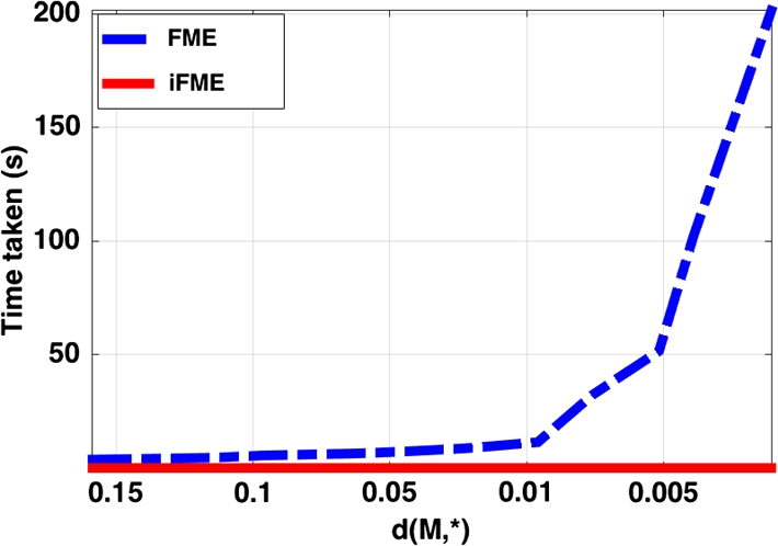
From the comparison plots in Fig. 7.4 we can see that iFME is very competitive in accuracy and much more efficient in execution time. We also present a comparison plots in Fig. 7.5 depicting the execution time taken by both the algorithms to achieve a prespecified error tolerance (with respect to the expectation of the distribution from which the samples are drawn). This plot suggests that to achieve a prespecified tolerance, iFME needs far less execution time compared to FME. Once again, all the time comparisons were performed on a 3.3 GHz desktop with quadcore Intel i7 processor and 24 GB RAM.

We now present an application to the atlas construction problem. Results on toy images taken from the MPEG-7 database using the proposed recursive FM computation technique are shown. Note that to compute the atlas, it is required to align the image data whose atlas we seek prior to computing the average. In this context we use the computationally efficient technique proposed in [52]. This technique involves picking an arbitrary reference image data set and aligning all the data to this reference. Then the alignment transformations between the reference and the rest of the images in the population are averaged. It was shown that this average transformation when applied to the chosen reference yields the atlas. For further details on this technique, we refer the reader to [52].
Two toy images were taken from the MPEG-7 database, and for each of these images, we generated four rotated images (highlighted in orange (mid gray in print version) in Fig. 7.6) and then computed the “mean image” (or atlas) of these rotated images (highlighted in red (dark gray in print version) in Fig. 7.6). The results clearly suggest that our approach gives an efficient way to compute atlas for images with planar rotations.

7.9 Conclusions
In this chapter we presented a recursive estimator for computing the Riemannian barycenter a.k.a. the Fréchet mean of manifold-valued data sets. Specifically, we developed the theory for two well-known and commonly encountered Riemannian manifolds, namely, the hypersphere Sn![]() and the special orthogonal group SO(n)
and the special orthogonal group SO(n)![]() . The common approach to estimating the FM from a set of data samples involves the application of Riemannian gradient descent to the Fréchet functional. This approach is not well suited for situations where data are acquired incrementally, that is, in an online fashion. In an online setting the Riemannian gradient descent proves to be inefficient both computationally and storagewise, since it requires computation of the Fréchet functional from scratch and thus requires the storage of all past data. In this chapter we presented a recursive FM estimator that does not require any optimization and achieves the computation of the FM estimate in a single pass over the data. We proved the weak consistency of the estimator for Sn
. The common approach to estimating the FM from a set of data samples involves the application of Riemannian gradient descent to the Fréchet functional. This approach is not well suited for situations where data are acquired incrementally, that is, in an online fashion. In an online setting the Riemannian gradient descent proves to be inefficient both computationally and storagewise, since it requires computation of the Fréchet functional from scratch and thus requires the storage of all past data. In this chapter we presented a recursive FM estimator that does not require any optimization and achieves the computation of the FM estimate in a single pass over the data. We proved the weak consistency of the estimator for Sn![]() and SO(n)
and SO(n)![]() . Further, we experimentally demonstrated that the estimator yields comparable accuracy to the Riemannian gradient descent algorithm. Several synthetic data and real-data experiments were presented showcasing the performance of the estimator in comparison to the Riemannian gradient descent technique for the FM computation and PG for the classification experiments with applications in neuroimaging. Our future work will focus on developing an FM estimator that uses intrinsic weights in the incremental updates, which will likely improve the convergence rate of the estimator.
. Further, we experimentally demonstrated that the estimator yields comparable accuracy to the Riemannian gradient descent algorithm. Several synthetic data and real-data experiments were presented showcasing the performance of the estimator in comparison to the Riemannian gradient descent technique for the FM computation and PG for the classification experiments with applications in neuroimaging. Our future work will focus on developing an FM estimator that uses intrinsic weights in the incremental updates, which will likely improve the convergence rate of the estimator.