
Probabilistic approaches to geometric statistics
Stochastic processes, transition distributions, and fiber bundle geometry
Stefan Sommer University of Copenhagen, Department of Computer Science, Copenhagen, Denmark
Abstract
We discuss construction of parametric families of intrinsically defined and geometrically natural probability distributions on manifolds, in particular, how to generalize the Euclidean normal distribution. This opens up for probabilistic formulations of concepts such as the mean value, covariance, and principal component analysis and general likelihood-based inference. The general idea is to use transition distributions of stochastic processes on manifolds to construct probabilistic models. For manifolds with connection, Gaussian-like distributions with nontrivial covariance structure can be defined via semielliptic diffusion processes in the frame bundle. On Lie groups diffusion processes can be similarly constructed using left or right trivialization to the Lie algebra. In both cases estimation of parameters of the underlying geometry or stochastic structure of the flows can be achieved either using most probable paths to the data, from matching moments of the generated distributions to sample moments of the data, or from Monte Carlo sampling of stochastic bridges to approximate transition distributions. We discuss the relation between geometry and noise structure and provide examples of how geometric statistics can be performed using stochastic flows.
Keywords
Probability distribution on a manifold; semielliptic diffusion process; Monte Carlo sampling; linear latent variable model; Euclidean principal component analysis; stochastic differential equation; Brownian motion on Riemannian manifold
10.1 Introduction
When generalizing Euclidean statistical concepts to manifolds, it is common to focus on particular properties of the Euclidean constructions and select those as the defining properties of the corresponding manifold generalization. This approach appears in many instances in geometric statistics, statistics of manifold-valued data. For example, the Fréchet mean [9] is the minimizer of the expected square distance to the data. It generalizes its Euclidean counterpart by using this least-squares criterion. Similarly, the principal component analysis (PCA) constructions discussed in Chapter 2 use the notion of linear subspaces from Euclidean space, generalizations of those to manifolds, and least-squares fit to data. Although one construction can often be defined via several equivalent characterizations in the Euclidean situation, curvature generally breaks such equivalences. For example, the mean value and PCA can in the Euclidean situation be formulated as maximum likelihood fits of normal distributions to the data resulting in the same constructions as the least-squares definitions. On curved manifolds the least-squares and maximum likelihood definitions give different results. Fitting probability distributions to data implies a shift of focus from the Riemannian distance as used in least-squares to an underlying probability model. We pursue such probabilistic approaches in this chapter.
The probabilistic viewpoint uses the concepts of likelihood-functions and parametric families of probability distributions. Generally, we search for a family of distributions μ(θ)![]() depending on the parameter θ with corresponding density function p(⋅;θ)
depending on the parameter θ with corresponding density function p(⋅;θ)![]() , from which we get a likelihood L(θ;y)=p(y;θ)
, from which we get a likelihood L(θ;y)=p(y;θ)![]() . With independent observations y1,…,yN
. With independent observations y1,…,yN![]() , we can then estimate the parameter by setting
, we can then estimate the parameter by setting
ˆθML=argmaxθN∏i=1L(θ;yi),
giving a sample maximum likelihood (ML) estimate of θ or, when a prior distribution p(θ)![]() for the parameters is available, the maximum a posteriori (MAP) estimate
for the parameters is available, the maximum a posteriori (MAP) estimate
ˆθMAP=argmaxθN∏i=1L(θ;yi)p(θ).

We can, for example, let the parameter θ denote a point m in M, and let μ(θ)![]() denote the normal distribution centered at m, in which case θML
denote the normal distribution centered at m, in which case θML![]() is a maximum likelihood mean. This viewpoint transfers the focus of manifold statistics from least-squares optimization to constructions of natural families of probability distributions μ(θ)
is a maximum likelihood mean. This viewpoint transfers the focus of manifold statistics from least-squares optimization to constructions of natural families of probability distributions μ(θ)![]() . A similar case arises when progressing beyond the mean to modeling covariance, data anisotropy, and principal components. The view here shifts from geodesic sprays and projections onto subspaces to the notion of covariance of a random variable. In a sense, we hide the complexity of the geometry in the construction of μ(θ)
. A similar case arises when progressing beyond the mean to modeling covariance, data anisotropy, and principal components. The view here shifts from geodesic sprays and projections onto subspaces to the notion of covariance of a random variable. In a sense, we hide the complexity of the geometry in the construction of μ(θ)![]() , which in turn implies that constructing such distributions is not always trivial.
, which in turn implies that constructing such distributions is not always trivial.
Throughout the chapter, we will take inspiration from and refer to the standard Euclidean linear latent variable model
y=m+Wx+ϵ
on Rd![]() with normally distributed latent variable x∼N(0,Idr)
with normally distributed latent variable x∼N(0,Idr)![]() , r≤d
, r≤d![]() and isotropic noise ϵ∼N(0,σ2Idd)
and isotropic noise ϵ∼N(0,σ2Idd)![]() . The marginal distribution of y is normal y∼N(m,Σ)
. The marginal distribution of y is normal y∼N(m,Σ)![]() as well with mean m and covariance Σ=WWT+σ2Idd
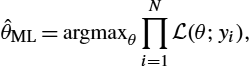
as well with mean m and covariance Σ=WWT+σ2Idd![]() . This simple model exemplifies many of the challenges when working with parametric probability distributions on manifolds: 1) Its definition relies on normal distributions with isotropic covariance for the distribution of x and ϵ. We describe two possible generalizations to manifolds of these, the Riemannian Normal law and the transition density of the Riemannian Brownian motion. 2) The model is additive, but on manifolds addition is only defined for tangent vectors. We handle this fact by defining probability models infinitesimally using stochastic differential equations. 3) The marginal distribution of y requires a way to translate the directions encoded in the matrix W to directions on the manifold. This can be done both in the tangent space of m, by using fiber bundles to move W with parallel transport, by using Lie group structure, or by referring to coordinate systems that in some cases have special meaning for the particular data at hand.
. This simple model exemplifies many of the challenges when working with parametric probability distributions on manifolds: 1) Its definition relies on normal distributions with isotropic covariance for the distribution of x and ϵ. We describe two possible generalizations to manifolds of these, the Riemannian Normal law and the transition density of the Riemannian Brownian motion. 2) The model is additive, but on manifolds addition is only defined for tangent vectors. We handle this fact by defining probability models infinitesimally using stochastic differential equations. 3) The marginal distribution of y requires a way to translate the directions encoded in the matrix W to directions on the manifold. This can be done both in the tangent space of m, by using fiber bundles to move W with parallel transport, by using Lie group structure, or by referring to coordinate systems that in some cases have special meaning for the particular data at hand.
The effect of including all these points is illustrated in Fig. 10.1. The linear Euclidean view of the data produced by tangent space principal component analysis (PCA) is compared to the linear Euclidean view provided by the infinitesimal probabilistic PCA model [34], which transports covariance parallel along the manifold. Because the infinitesimal model does not linearize to a single tangent space and because of the built-in notion of data anisotropy, infinitesimal covariance, the provided Euclidean view gives a better representation of the data variability.

 with added minor variation orthogonal to the circle. The sphere is colored by the density of the distribution, the transition density of the underlying stochastic process. (Right) Red crosses (gray in print version): Data mapped to the tangent space of the north pole using the standard tangent principal component analysis (PCA) linearization. Variation orthogonal to the great circle is overestimated because the curvature of the sphere lets geodesics (red (gray in print version) curve and line) leave high-density areas of the distribution. Black dots: Corresponding linearization of the data using the infinitesimal probabilistic PCA model [34]. The black curve represents the expectation over samples of the latent process conditioned on the same observation as the red (gray in print version) curve. The corresponding path shown on the left figure clearly is attracted to the high-density area of the distribution contrary to the geodesic. The orthogonal variation is not overestimated, and the Euclidean view provides a better representation of the data variability.
We start in section 10.2 by discussing two ways to pursue construction of μ(θ)![]() via density functions and from transition distributions of stochastic processes. We exemplify the former with the probabilistic principal geodesic analysis (PPGA) generalization of manifold PCA, and the later with maximum likelihood means and an infinitesimal version of probabilistic PCA. In section 10.3, we discuss the most important stochastic process on manifolds, the Brownian motion, and its transition distribution, both in the Riemannian manifold case and when Lie group structure is present. In section 10.4, we describe aspects of fiber bundle geometry necessary for the construction of stochastic processes with infinitesimal covariance as pursued in section 10.5. The fiber bundle construction can be seen as a way to handle the lack of global coordinate system. Whereas it touches concepts beyond the standard set of Riemannian geometric notions discussed in chapter 1, it provides intrinsic geometric constructions that are very useful from a statistical viewpoint. We use this in section 10.6 to define statistical concepts as maximum likelihood parameter fits to data and in section 10.7 to perform parameter estimation. In section 10.8, we discuss advanced concepts arising from fiber bundle geometry, including interpretation of the curvature tensor, sub-Riemannian frame-bundle geometry, and examples of flows using additional geometric structure present in specific models of shape.
via density functions and from transition distributions of stochastic processes. We exemplify the former with the probabilistic principal geodesic analysis (PPGA) generalization of manifold PCA, and the later with maximum likelihood means and an infinitesimal version of probabilistic PCA. In section 10.3, we discuss the most important stochastic process on manifolds, the Brownian motion, and its transition distribution, both in the Riemannian manifold case and when Lie group structure is present. In section 10.4, we describe aspects of fiber bundle geometry necessary for the construction of stochastic processes with infinitesimal covariance as pursued in section 10.5. The fiber bundle construction can be seen as a way to handle the lack of global coordinate system. Whereas it touches concepts beyond the standard set of Riemannian geometric notions discussed in chapter 1, it provides intrinsic geometric constructions that are very useful from a statistical viewpoint. We use this in section 10.6 to define statistical concepts as maximum likelihood parameter fits to data and in section 10.7 to perform parameter estimation. In section 10.8, we discuss advanced concepts arising from fiber bundle geometry, including interpretation of the curvature tensor, sub-Riemannian frame-bundle geometry, and examples of flows using additional geometric structure present in specific models of shape.
We aim with the chapter for providing an overview of aspects of probabilistic statistics on manifolds in an accessible way. This implies that mathematical details on the underlying geometry and stochastic analysis are partly omitted. We provide references to the papers where the presented material was introduced in each section, and we include references for further reading by the end of the chapter. The code for the presented models and parameter estimation algorithms discussed in this chapter are available in the Theano Geometry library https://bitbucket.com/stefansommer/theanogeometry, see also [16,15].
10.2 Parametric probability distributions on manifolds
We here discuss two ways of defining families of probability distributions on a manifold: directly from a density function, or as the transition distribution of a stochastic process. We exemplify their use with the probabilistic PGA generalization of Euclidean PCA and an infinitesimal counterpart based on an underlying stochastic process.
10.2.1 Probabilistic PCA
Euclidean principal component analysis (PCA) is traditionally defined as a fit of best approximating linear subspaces of a given dimension to data, either by maximizing variance
ˆW=argmaxW∈O(Rr,Rd)N∑i=1‖WWTyi‖2

of the centered data y1,…,yN![]() projected to r-dimensional subspaces of Rd
projected to r-dimensional subspaces of Rd![]() represented here by orthonormal matrices W∈O(Rr,Rd)
represented here by orthonormal matrices W∈O(Rr,Rd)![]() of rank r or by minimizing residual errors
of rank r or by minimizing residual errors
ˆW=argminW∈O(Rr,Rd)N∑i=1‖yi−WWTyi‖2

between the observations and their projections to the subspace. We see that fundamental for this construction is the notion of linear subspace, projections to linear subspaces, and squared distances. The dimension r of the fitted subspace determines the number of principal components.
PCA can however also be defined from a probabilistic viewpoint [37,29]. The approach is here to fit the latent variable model (10.3) with W of fixed rank r. The conditional distribution of the data given the latent variable x∈Rr![]() is normal
is normal
y|x∼N(m+Wx,σ2I).
With x normally distributed N(0,Idr)![]() and noise ϵ∼N(0,σ2Idd)
and noise ϵ∼N(0,σ2Idd)![]() , the marginal distribution of y is y∼N(m,Σ)
, the marginal distribution of y is y∼N(m,Σ)![]() with Σ=WWT+σ2Idd
with Σ=WWT+σ2Idd![]() .
.
The Euclidean principal components of the data are here interpreted as the conditional distribution x|yi![]() of x given the data yi
of x given the data yi![]() . From the data conditional distribution, a single quantity representing yi
. From the data conditional distribution, a single quantity representing yi![]() can be obtained by taking expectation xi:=E[x|yi]=(WTW+σ2I)−1WT(yi−m)
can be obtained by taking expectation xi:=E[x|yi]=(WTW+σ2I)−1WT(yi−m)![]() . The parameters of the model m, W, σ can be found by maximizing the likelihood
. The parameters of the model m, W, σ can be found by maximizing the likelihood
L(W,σ,m;y)=|2πΣ|−12e−12(y−m)TΣ−1(y−m)).
Up to rotation, the ML fit of W is given by ˆWML=ˆUr(ˆΛ−σ2Idd)1/2![]() , where ˆΛ=diag(ˆλ1,…,ˆλr)
, where ˆΛ=diag(ˆλ1,…,ˆλr)![]() , ˆUr
, ˆUr![]() contains the first r principal eigenvectors of the sample covariance matrix of yi
contains the first r principal eigenvectors of the sample covariance matrix of yi![]() in the columns, and ˆλ1,…,ˆλr
in the columns, and ˆλ1,…,ˆλr![]() are the corresponding eigenvalues.
are the corresponding eigenvalues.
10.2.2 Riemannian normal distribution and probabilistic PGA
We saw in chapter 2 the Normal law or Riemannian normal distribution defined via its density
p(y;m,σ2)=C(m,σ2)−1e−dist(m,y)22σ2
with normalization constant C(m,σ2)![]() and the parameter σ2
and the parameter σ2![]() controlling the dispersion of the distribution. The density is given with respect to the volume measure dVg
controlling the dispersion of the distribution. The density is given with respect to the volume measure dVg![]() on M
on M![]() , so that the actual distribution is p(⋅;m,σ2)dVg
, so that the actual distribution is p(⋅;m,σ2)dVg![]() . Because of the use of the Riemannian distance function, the distribution is at first sight related to a normal distribution N(0,σ2Idd)
. Because of the use of the Riemannian distance function, the distribution is at first sight related to a normal distribution N(0,σ2Idd)![]() in TmM
in TmM![]() ; however, its definition with respect to the measure dVg
; however, its definition with respect to the measure dVg![]() implies that it differs from the density of the normal distribution at each point of TmM
implies that it differs from the density of the normal distribution at each point of TmM![]() by the square root determinant of the metric |g|12
by the square root determinant of the metric |g|12![]() . The isotropic precision/concentration matrix σ−2Idd
. The isotropic precision/concentration matrix σ−2Idd![]() can be exchanged with a more general concentration matrix in TmM
can be exchanged with a more general concentration matrix in TmM![]() . The distribution maximizes the entropy for fixed parameters (m,Σ)
. The distribution maximizes the entropy for fixed parameters (m,Σ)![]() [26].
[26].
This distribution is used in [39] to generalize Euclidean PPCA. Here the distribution of the latent variable x is normal in TmM![]() , x is mapped to M
, x is mapped to M![]() using Expm
using Expm![]() , and the conditional distribution y|x
, and the conditional distribution y|x![]() of the observed data y given x is Riemannian normal p(y;Expmx,σ2)dVg
of the observed data y given x is Riemannian normal p(y;Expmx,σ2)dVg![]() . The matrix W models the square root covariance Σ=WWT
. The matrix W models the square root covariance Σ=WWT![]() of the latent variable x in TmM
of the latent variable x in TmM![]() . The model is called probabilistic principal geodesic analysis (PPGA).
. The model is called probabilistic principal geodesic analysis (PPGA).
10.2.3 Transition distributions and stochastic differential equations
Instead of mapping latent variables from TmM![]() to M
to M![]() using the exponential map, we can take an infinitesimal approach and only map infinitesimal displacements to the manifold, thereby avoiding the use of Expm
using the exponential map, we can take an infinitesimal approach and only map infinitesimal displacements to the manifold, thereby avoiding the use of Expm![]() and the implicit linearization coming from the use of a single tangent space. The idea is to create probability distributions as solutions to stochastic differential equations, SDEs. In Euclidean space, SDEs are usually written on the form
and the implicit linearization coming from the use of a single tangent space. The idea is to create probability distributions as solutions to stochastic differential equations, SDEs. In Euclidean space, SDEs are usually written on the form
dy(t)=b(t,y(t))dt+a(t,y(t))dx(t),
where a:R×Rd→Rd×d![]() is the diffusion field modeling the local diffusion of the process, and b:R×Rd→Rd
is the diffusion field modeling the local diffusion of the process, and b:R×Rd→Rd![]() models the deterministic drift. The process x(t)
models the deterministic drift. The process x(t)![]() of which we multiply the infinitesimal increments dx(t)
of which we multiply the infinitesimal increments dx(t)![]() on a is a semimartingale. For our purposes, we can assume that it is a standard Brownian motion, often written W(t)
on a is a semimartingale. For our purposes, we can assume that it is a standard Brownian motion, often written W(t)![]() or B(t)
or B(t)![]() . Solutions to (10.9) are defined by an integral equation that discretized in time takes the form
. Solutions to (10.9) are defined by an integral equation that discretized in time takes the form
y(ti)=y(0)+i−1∑j=1b(tj,y(tj))(tj+1−tj)+a(tj,y(tj))(x(tj+1)−x(tj)).
This is called an Itô equation. Alternatively, we can use the Fisk–Stratonovich solution
y(ti)=y(0)+i−1∑j=1b(t⁎j,y(t⁎j))(tj+1−tj)+a(t⁎j,y(t⁎j))(x(tj+1)−x(tj))

where t⁎j=(tj+1−tj)/2![]() , that is, the integrand is evaluated at the midpoint. Notationally, Fisk–Stratonovich SDEs, often just called Stratonovich SDEs, are distinguished from Itô SDEs by adding ∘ in the diffusion term a(t,y(t))∘dx(t)
, that is, the integrand is evaluated at the midpoint. Notationally, Fisk–Stratonovich SDEs, often just called Stratonovich SDEs, are distinguished from Itô SDEs by adding ∘ in the diffusion term a(t,y(t))∘dx(t)![]() in (10.9). The main purpose here of using Stratonovich SDEs is that solutions obey the ordinary chain rule of differentiation and therefore map naturally between manifolds.
in (10.9). The main purpose here of using Stratonovich SDEs is that solutions obey the ordinary chain rule of differentiation and therefore map naturally between manifolds.
A solution y(t)![]() to an SDE is a t-indexed family of probability distributions. If we fix a time T>0
to an SDE is a t-indexed family of probability distributions. If we fix a time T>0![]() , then the transition distribution y(T)
, then the transition distribution y(T)![]() denotes the distribution of endpoints of sample paths y(ω)(t)
denotes the distribution of endpoints of sample paths y(ω)(t)![]() , where ω is a particular random event. We can thus generate distributions in this way and set μ(θ)=y(T)
, where ω is a particular random event. We can thus generate distributions in this way and set μ(θ)=y(T)![]() , where the parameters θ now control the dynamics of the process via the SDE, particularly the drift b, the diffusion field a, and the starting point y0
, where the parameters θ now control the dynamics of the process via the SDE, particularly the drift b, the diffusion field a, and the starting point y0![]() of the process.
of the process.
The use of SDEs fits the differential structure of manifolds well because SDEs are defined infinitesimally. However, because we generally do not have global coordinate systems to write up an SDE as in (10.9), defining SDEs on manifolds takes some work. We will see several examples of this in the sections below.
Particularly, we will define an SDE that reformulates (10.3) as a time-sequence of random steps, where the latent variable x will be replaced by a latent process x(t)![]() , where the covariance W will be parallel transported over M
, where the covariance W will be parallel transported over M![]() . This process will again have parameters (m,W,σ)
. This process will again have parameters (m,W,σ)![]() . We define the distribution μ(m,W,σ)
. We define the distribution μ(m,W,σ)![]() by setting μ(m,W,σ)=y(T)
by setting μ(m,W,σ)=y(T)![]() , and we then assume that the observed data y1,…,yN
, and we then assume that the observed data y1,…,yN![]() have marginal distribution yi∼μ(m,W,σ)
have marginal distribution yi∼μ(m,W,σ)![]() . Note that y(T)
. Note that y(T)![]() is a distribution, whereas yi
is a distribution, whereas yi![]() , i=1,…,N
, i=1,…,N![]() , denote the data.
, denote the data.
Let p(yi;m,W,σ)![]() denote the density of the distribution μ(m,W,σ)
denote the density of the distribution μ(m,W,σ)![]() with respect to a fixed measure. As in the PPCA situation, we then have a likelihood for the model
with respect to a fixed measure. As in the PPCA situation, we then have a likelihood for the model
L(m,W,σ;yi)=p(yi;m,W,σ),
and we can optimize for the ML estimate ˆθ=(ˆm,ˆW,ˆσ)![]() . Again, similarly to the PPCA construction, we get the generalization of the principal components by conditioning the latent process on the data: xi,t:=x(t)|y(T)=yi
. Again, similarly to the PPCA construction, we get the generalization of the principal components by conditioning the latent process on the data: xi,t:=x(t)|y(T)=yi![]() . The picture here is that among all sample paths y(ω)(t)
. The picture here is that among all sample paths y(ω)(t)![]() , we single out those hitting yi
, we single out those hitting yi![]() at time T and consider the corresponding realizations of the latent process x(ω)(t)
at time T and consider the corresponding realizations of the latent process x(ω)(t)![]() a representation of the data.
a representation of the data.
Fig. 10.1 displays the result of pursuing this construction compared to tangent space PCA. Because the anisotropic covariance is now transported with the process instead of being tied to a single tangent space, the curvature of the sphere is in a sense incorporated into the model, and the linear view of the data xi,t![]() , particularly the endpoints xi:=xi,T
, particularly the endpoints xi:=xi,T![]() , provide an improved picture of the data variation on the manifold.
, provide an improved picture of the data variation on the manifold.
Below, we will make the construction of the underlying stochastic process precise and present other examples of geometrically natural processes that allow for generating geometrically natural families of probability distributions μ(θ)![]() .
.
10.3 The Brownian motion
In Euclidean space the normal distribution N(0,Idd)![]() is often defined in terms of its density function. This view leads naturally to the Riemannian normal distribution or the normal law (10.8). A different characterization [10] is as the transition distribution of an isotropic diffusion processes, the heat equation. Here the density is the solution to the partial differential equation
is often defined in terms of its density function. This view leads naturally to the Riemannian normal distribution or the normal law (10.8). A different characterization [10] is as the transition distribution of an isotropic diffusion processes, the heat equation. Here the density is the solution to the partial differential equation
∂tp(t,y)=12Δp(t,y),y∈Rk,
where p:R×Rk→R![]() is a real-valued function, Δ is the Laplace differential operator Δ=∂2y1+⋯+∂2yk
is a real-valued function, Δ is the Laplace differential operator Δ=∂2y1+⋯+∂2yk![]() . If (10.13) is started at time t=0
. If (10.13) is started at time t=0![]() with p(y)=δm(y)
with p(y)=δm(y)![]() , that is, the indicator function taking the value 1 only when y=m
, that is, the indicator function taking the value 1 only when y=m![]() , the time t=1
, the time t=1![]() solution is the density of the normal distribution N(m,Idk)
solution is the density of the normal distribution N(m,Idk)![]() . We can think of a point-sourced heat distribution starting at m and diffusing through the domain from time t=0
. We can think of a point-sourced heat distribution starting at m and diffusing through the domain from time t=0![]() to t=1
to t=1![]() .
.
The heat flow can be characterized probabilistically from a stochastic process, the Brownian motion B(t)![]() . When started at m at time t=0
. When started at m at time t=0![]() , a solution p to the heat flow equation (10.13) describes the density of the random variable B(t)
, a solution p to the heat flow equation (10.13) describes the density of the random variable B(t)![]() for each t. Therefore, we again regain the density of the normal distribution N(m,Idk)
for each t. Therefore, we again regain the density of the normal distribution N(m,Idk)![]() as the density of B(1)
as the density of B(1)![]() . The heat flow and the Brownian motion view of the normal distribution generalize naturally to the manifold situation. Because the Laplacian is a differential operator and because the Brownian motion is constructed from random infinitesimal increments, the construction is an infinitesimal construction as discussed in section 10.2.3.
. The heat flow and the Brownian motion view of the normal distribution generalize naturally to the manifold situation. Because the Laplacian is a differential operator and because the Brownian motion is constructed from random infinitesimal increments, the construction is an infinitesimal construction as discussed in section 10.2.3.
Whereas in this section we focus on aspects of the Brownian motion, we will later see that solutions y(t)![]() to the SDE dy(t)=WdB(t)
to the SDE dy(t)=WdB(t)![]() with more general matrices W in addition allows modeling covariance in the normal distribution, even in the manifold situation, using the fact that in the Euclidean situation, y(1)∼N(m,Σ)
with more general matrices W in addition allows modeling covariance in the normal distribution, even in the manifold situation, using the fact that in the Euclidean situation, y(1)∼N(m,Σ)![]() when Σ=WWT
when Σ=WWT![]() .
.
10.3.1 Brownian motion on Riemannian manifolds
A Riemannian metric g defines the Laplace–Beltrami operator Δg![]() that generalizes the usual Euclidean Laplace operator used in (10.13). The operator is defined on real-valued functions by Δgf=divgradgfg
that generalizes the usual Euclidean Laplace operator used in (10.13). The operator is defined on real-valued functions by Δgf=divgradgfg![]() . When e1,…,ed
. When e1,…,ed![]() is an orthonormal basis for TyM
is an orthonormal basis for TyM![]() , it has the expression Δgf(y)=∑i=1d∇2yf(ei,ei)
, it has the expression Δgf(y)=∑i=1d∇2yf(ei,ei)![]() when evaluated at y similarly to the Euclidean Laplacian. The expression ∇2yf(ei,ei)
when evaluated at y similarly to the Euclidean Laplacian. The expression ∇2yf(ei,ei)![]() denotes the Hessian ∇2y
denotes the Hessian ∇2y![]() evaluated at the pair of vectors (ei,ei)
evaluated at the pair of vectors (ei,ei)![]() . The heat equation on M
. The heat equation on M![]() is the partial differential equation defined from the Laplace–Beltrami operator by
is the partial differential equation defined from the Laplace–Beltrami operator by
∂tp(t,y)=12Δgp(t,y),y∈M.
With initial condition p(0,⋅)![]() at t=0
at t=0![]() being the indicator function δm(y)
being the indicator function δm(y)![]() , the solution is called the heat kernel and written p(t,m,y)
, the solution is called the heat kernel and written p(t,m,y)![]() when evaluated at y∈M
when evaluated at y∈M![]() . The heat equation again models point sourced heat flows starting at m and diffusing through the medium with the Laplace–Beltrami operator now ensuring that the flow is adapted to the nonlinear geometry. The heat kernel is symmetric in that p(t,m,y)=p(t,y,m)
. The heat equation again models point sourced heat flows starting at m and diffusing through the medium with the Laplace–Beltrami operator now ensuring that the flow is adapted to the nonlinear geometry. The heat kernel is symmetric in that p(t,m,y)=p(t,y,m)![]() and satisfies the semigroup property
and satisfies the semigroup property
p(t+s,m,y)=∫Mp(t,m,z)p(s,z,y)dVg(z).

Similarly to the Euclidean situation, we can recover the heat kernel from a diffusion process on M![]() , the Brownian motion. The Brownian motion on Riemannian manifolds and Lie groups with a Riemannian metric can be constructed in several ways: Using charts, by embedding in a Euclidean space, or using left/right invariance as we pursue in this section. A particular important construction here is the Eells–Elworthy–Malliavin construction of Brownian motion that uses a fiber bundle of the manifold to define an SDE for the Brownian motion. We will use this construction in section 10.4 and through the rest of the chapter.
, the Brownian motion. The Brownian motion on Riemannian manifolds and Lie groups with a Riemannian metric can be constructed in several ways: Using charts, by embedding in a Euclidean space, or using left/right invariance as we pursue in this section. A particular important construction here is the Eells–Elworthy–Malliavin construction of Brownian motion that uses a fiber bundle of the manifold to define an SDE for the Brownian motion. We will use this construction in section 10.4 and through the rest of the chapter.
The heat kernel p(t,m,y)![]() is related to a Brownian motion x(t)
is related to a Brownian motion x(t)![]() on M
on M![]() by its transition density, that is,
by its transition density, that is,
Pm(x(t)∈C)=∫Cp(t,m,y)dVg(y)
for subsets C⊂M![]() . If M
. If M![]() is assumed compact, it can be shown that it is stochastically complete, which implies that the Brownian motion exists for all time and that ∫Mp(t,m,y)dVg(y)=1
is assumed compact, it can be shown that it is stochastically complete, which implies that the Brownian motion exists for all time and that ∫Mp(t,m,y)dVg(y)=1![]() for all t>0
for all t>0![]() . If M
. If M![]() is not compact, the long time existence can be ensured by, for example, bounding the Ricci curvature of M
is not compact, the long time existence can be ensured by, for example, bounding the Ricci curvature of M![]() from below; see, for example, [7]. In coordinates, a solution y(t)
from below; see, for example, [7]. In coordinates, a solution y(t)![]() to the Itô SDE
to the Itô SDE
dy(t)i=b(y(t))dt+√g(y(t))−1idB(t)
is a Brownian motion on M![]() [13]. Here B(t)
[13]. Here B(t)![]() is a Euclidean Rd
is a Euclidean Rd![]() -valued Brownian motion, the diffusion field √g(y(t))−1
-valued Brownian motion, the diffusion field √g(y(t))−1![]() is a square root of the cometric tensor g(y(t))ij
is a square root of the cometric tensor g(y(t))ij![]() , and the drift b(y(t))
, and the drift b(y(t))![]() is the contraction −12g(y(t))klΓ(y(t))kl
is the contraction −12g(y(t))klΓ(y(t))kl![]() of the metric and the Christoffel symbols Γkli
of the metric and the Christoffel symbols Γkli![]() . Fig. 10.2 shows sample paths from a Brownian motion on the sphere S2
. Fig. 10.2 shows sample paths from a Brownian motion on the sphere S2![]() .
.
 .
.10.3.2 Lie groups
With a left-invariant metric on a Lie group G (see chapter 1), the Laplace–Beltrami operator takes the form Δf(x)=Δ(Lyf)(y−1x)![]() for all x,y∈G
for all x,y∈G![]() . By left-translating to the identity the operator thus needs only be computed at x=e
. By left-translating to the identity the operator thus needs only be computed at x=e![]() , that is, at the Lie algebra g
, that is, at the Lie algebra g![]() . Like the Laplace–Beltrami operator, the heat kernel is left-invariant [21] when the metric is left-invariant. Similar invariance happens in the right-invariant case.
. Like the Laplace–Beltrami operator, the heat kernel is left-invariant [21] when the metric is left-invariant. Similar invariance happens in the right-invariant case.
Let e1,…,ed![]() be an orthonormal basis for g
be an orthonormal basis for g![]() , so that Xi(y)=(Ly)⁎(ei)
, so that Xi(y)=(Ly)⁎(ei)![]() is an orthonormal set of vector fields on G. Let Cijk
is an orthonormal set of vector fields on G. Let Cijk![]() denote the structure coefficients given by
denote the structure coefficients given by
[Xj,Xk]=CijkXi,
and let B(t)![]() be a standard Brownian motion on Rd
be a standard Brownian motion on Rd![]() . Then the solution y(t)
. Then the solution y(t)![]() of the Stratonovich differential equation
of the Stratonovich differential equation
dy(t)=−12∑j,iCjijXi(y(t))dt+Xi(y(t))∘dB(t)i

is a Brownian motion on G. Fig. 10.3 visualizes a sample path of B(t)![]() and the corresponding sample of y(t)
and the corresponding sample of y(t)![]() on the group SO(3)
on the group SO(3)![]() . When the metric on g
. When the metric on g![]() is in addition Ad-invariant, the drift term vanishes leaving only the multiplication of the Brownian motion increments on the basis.
is in addition Ad-invariant, the drift term vanishes leaving only the multiplication of the Brownian motion increments on the basis.

 . (Right) The corresponding sample path y(ω)(t) of the SO(3)-valued process (10.17) visualized by the action of rotation y.(e1,e2,e3), y ∈ SO(3) on three basis vectors e1, e2, e3 (red/green/blue) (gray/light gray/dark gray in print version) for R3.
The left-invariant fields Xi(y)![]() here provide a basis for the tangent space at y that in (10.17) is used to map increments of the Euclidean Brownian motion B(t)
here provide a basis for the tangent space at y that in (10.17) is used to map increments of the Euclidean Brownian motion B(t)![]() to TyG
to TyG![]() . The fact that Xi
. The fact that Xi![]() are defined globally allows this construction to specify the evolution of the process at all points of G without referring to charts as in (10.15). We will later on explore a different approach to obtain a structure much like the Lie group fields Xi
are defined globally allows this construction to specify the evolution of the process at all points of G without referring to charts as in (10.15). We will later on explore a different approach to obtain a structure much like the Lie group fields Xi![]() but on general manifolds, where we do not have globally defined continuous and nonzero vector fields. This allows us to write the Brownian motion globally as in the Lie group case.
but on general manifolds, where we do not have globally defined continuous and nonzero vector fields. This allows us to write the Brownian motion globally as in the Lie group case.
10.4 Fiber bundle geometry
In the Lie group case, Brownian motion can be constructed by mapping a Euclidean process B(t)![]() to the group to get the process y(t)
to the group to get the process y(t)![]() . This construction uses the set of left- (or right)-vector fields Xi(y)=(Ly)⁎(ei)
. This construction uses the set of left- (or right)-vector fields Xi(y)=(Ly)⁎(ei)![]() that are globally defined and, with a left-invariant metric, orthonormal. Globally defined maps from a manifold to its tangent bundle are called sections, and manifolds that support sections of the tangent bundle that at each point form a basis for the tangent space are called parallelizable, a property that Lie groups possess but not manifolds in general. The sphere S2
that are globally defined and, with a left-invariant metric, orthonormal. Globally defined maps from a manifold to its tangent bundle are called sections, and manifolds that support sections of the tangent bundle that at each point form a basis for the tangent space are called parallelizable, a property that Lie groups possess but not manifolds in general. The sphere S2![]() is an example: The hairy-ball theorem asserts that no continuous nowhere vanishing vector fields exist on S2
is an example: The hairy-ball theorem asserts that no continuous nowhere vanishing vector fields exist on S2![]() . Thus we have no chance of finding a set of nonvanishing global vector fields, not to mention a set of fields constituting an orthonormal basis, which we can use to write an SDE similar to (10.17).
. Thus we have no chance of finding a set of nonvanishing global vector fields, not to mention a set of fields constituting an orthonormal basis, which we can use to write an SDE similar to (10.17).
A similar issue arises when generalizing the latent variable model (10.3). We can use the tangent space at m to model the latent variables x, map to the manifold using the Riemannian exponential map Expm![]() , and use the Riemannian Normal law to model the conditional distribution y|x
, and use the Riemannian Normal law to model the conditional distribution y|x![]() . However, if we wish to avoid the linearization implied by using the tangent space at m, then we need to convert (10.3) from using addition of the vectors x, W, and ϵ to work infinitesimally, to use addition of infinitesimal steps in tangent spaces, and to transport W between these tangent spaces. We can achieve this by converting (10.3) to the SDE
. However, if we wish to avoid the linearization implied by using the tangent space at m, then we need to convert (10.3) from using addition of the vectors x, W, and ϵ to work infinitesimally, to use addition of infinitesimal steps in tangent spaces, and to transport W between these tangent spaces. We can achieve this by converting (10.3) to the SDE
dy(t)=Wdx(t)+dϵ(t)
started at m, where x(t)![]() is now a Euclidean Brownian motion, and ϵ(t)
is now a Euclidean Brownian motion, and ϵ(t)![]() is a Euclidean Brownian motion scaled by σ. The latent process x(t)
is a Euclidean Brownian motion scaled by σ. The latent process x(t)![]() here takes the place of the latent variable x in (10.3) with x(1)
here takes the place of the latent variable x in (10.3) with x(1)![]() and x having the same distribution N(0,Idd)
and x having the same distribution N(0,Idd)![]() . We write x(t)
. We write x(t)![]() instead of B(t)
instead of B(t)![]() to emphasize this. Similarly, the noise process ϵ(t)
to emphasize this. Similarly, the noise process ϵ(t)![]() takes the place of ϵ with ϵ(1)
takes the place of ϵ with ϵ(1)![]() and ϵ having the same distribution N(0,σ2Idd)
and ϵ having the same distribution N(0,σ2Idd)![]() . In Euclidean space, the transition distribution of this SDE will be equal to the marginal distribution of y in (10.3), that is, y1∼N(m,Σ)
. In Euclidean space, the transition distribution of this SDE will be equal to the marginal distribution of y in (10.3), that is, y1∼N(m,Σ)![]() and Σ=WWT+σ2Idd
and Σ=WWT+σ2Idd![]() . On the manifold we however need to handle the fact that the matrix W is defined at first only in the tangent space TmM
. On the manifold we however need to handle the fact that the matrix W is defined at first only in the tangent space TmM![]() . The natural way to move W to tangent spaces nearby m is by parallel transport of the vectors constituting the columns of W. This reflects the Euclidean situation where W is independent of x(t)
. The natural way to move W to tangent spaces nearby m is by parallel transport of the vectors constituting the columns of W. This reflects the Euclidean situation where W is independent of x(t)![]() and hence spatially stationary. However, parallel transport is tied to paths, so the result will be a transport of W that is now different for each sample path realization of (10.18). This fact is beautifully handled with the Eells–Elworthy–Malliavin [6] construction of Brownian motion. We outline this construction below. For this, we first need some important notions from fiber bundle geometry.
and hence spatially stationary. However, parallel transport is tied to paths, so the result will be a transport of W that is now different for each sample path realization of (10.18). This fact is beautifully handled with the Eells–Elworthy–Malliavin [6] construction of Brownian motion. We outline this construction below. For this, we first need some important notions from fiber bundle geometry.
10.4.1 The frame bundle
A fiber bundle over a manifold M is a manifold E with a map π:E→M![]() , called the projection, such that for sufficiently small neighborhoods U⊂M
, called the projection, such that for sufficiently small neighborhoods U⊂M![]() , the preimage π−1(U)
, the preimage π−1(U)![]() can be written as a product π−1≃U×F
can be written as a product π−1≃U×F![]() between U and a manifold F, the fiber. When the fibers are vector spaces, fiber bundles are called vector bundles. The most commonly occurring vector bundle is the tangent bundle TM. Recall that a tangent vector always lives in a tangent space at a point in M, that is, v∈TyM
between U and a manifold F, the fiber. When the fibers are vector spaces, fiber bundles are called vector bundles. The most commonly occurring vector bundle is the tangent bundle TM. Recall that a tangent vector always lives in a tangent space at a point in M, that is, v∈TyM![]() . The map π(v)=y
. The map π(v)=y![]() is the projection, and the fiber π−1(y)
is the projection, and the fiber π−1(y)![]() of the point y is the vector space TyM
of the point y is the vector space TyM![]() , which is isomorphic to Rd
, which is isomorphic to Rd![]() .
.
Consider now basis vectors W1,…,Wd![]() for TyM
for TyM![]() . As an ordered set (W1,…,Wd)
. As an ordered set (W1,…,Wd)![]() , the vectors are in combination called a frame. The frame bundle FM
, the vectors are in combination called a frame. The frame bundle FM![]() is a fiber bundle over M such that the fibers π−1(y)
is a fiber bundle over M such that the fibers π−1(y)![]() are sets of frames. Therefore a point u∈FM
are sets of frames. Therefore a point u∈FM![]() consists of a collection of basis vectors (W1,…,Wd)
consists of a collection of basis vectors (W1,…,Wd)![]() and the base point y∈M
and the base point y∈M![]() of which W1,…,Wd
of which W1,…,Wd![]() make up a basis for TyM
make up a basis for TyM![]() . We can use the local product structure of frame bundles to locally write u=(y,W)
. We can use the local product structure of frame bundles to locally write u=(y,W)![]() where y∈M
where y∈M![]() as W1,…,Wd
as W1,…,Wd![]() are the basis vectors. Often, we denote the basis vectors in u just u1,…,ud
are the basis vectors. Often, we denote the basis vectors in u just u1,…,ud![]() . The frame bundle has interesting geometric properties, which we will use through the chapter. The frame bundle of S2
. The frame bundle has interesting geometric properties, which we will use through the chapter. The frame bundle of S2![]() is illustrated in Fig. 10.4.
is illustrated in Fig. 10.4.

 of the sphere S2 illustrated by its representation as the principal bundle GL(R2,TS2)
 . A point u∈FS2
 can be seen as a linear map from R2
 (left) to the tangent space TxS2
 of the point y = π(u) (right). The standard basis (e1,e2) for R2 maps to a basis (u1,u2), ui = uei for TyS2
 because the frame bundle element u defines a linear map R2→TyS2
 . The vertical subbundle of the tangent bundle TFS2
 consists of derivatives of paths in FS2 that only change the frame, that is, π(u) is fixed. Vertical vectors act by rotation of the basis vectors as illustrated by the rotation of the basis seen along the vertical line. The horizontal subbundle, which can be seen as orthogonal to the vertical subbundle, arises from parallel transporting vectors in the frame u along paths on S2.
10.4.2 Horizontality
The frame bundle, being a manifold, itself has a tangent bundle TFM![]() with derivatives ˙u(t)
with derivatives ˙u(t)![]() of paths u(t)∈FM
of paths u(t)∈FM![]() being vectors in Tu(t)FM
being vectors in Tu(t)FM![]() . We can use the fiber bundle structure to split TFM
. We can use the fiber bundle structure to split TFM![]() and thereby define two different types of infinitesimal movements in FM
and thereby define two different types of infinitesimal movements in FM![]() . First, a path u(t)
. First, a path u(t)![]() can vary solely in the fiber direction meaning that for some y∈M
can vary solely in the fiber direction meaning that for some y∈M![]() , π(u(t))=y
, π(u(t))=y![]() for all t. Such a path is called vertical. At a point u∈FM
for all t. Such a path is called vertical. At a point u∈FM![]() the derivative of the path lies in the linear subspace VuFM
the derivative of the path lies in the linear subspace VuFM![]() of TuFM
of TuFM![]() called the vertical subspace. For each y, VuFM
called the vertical subspace. For each y, VuFM![]() is a d2
is a d2![]() -dimensional manifold. It corresponds to changes of the frame, the basis vectors for TyM
-dimensional manifold. It corresponds to changes of the frame, the basis vectors for TyM![]() , while the base point y is kept fixed. FM
, while the base point y is kept fixed. FM![]() is a (d+d2)
is a (d+d2)![]() -dimensional manifold, and the subspace containing the remaining d dimensions of TuFM
-dimensional manifold, and the subspace containing the remaining d dimensions of TuFM![]() is in a particular sense separate from the vertical subspace. It is therefore called the horizontal subspace HuFM
is in a particular sense separate from the vertical subspace. It is therefore called the horizontal subspace HuFM![]() . Just as tangent vectors in VuFM
. Just as tangent vectors in VuFM![]() model changes only in the frame keeping y fixed, the horizontal subspace models changes of y keeping, in a sense, the frame fixed. However, frames are tied to tangent spaces, so we need to define what is meant by keeping the frame fixed. When M
model changes only in the frame keeping y fixed, the horizontal subspace models changes of y keeping, in a sense, the frame fixed. However, frames are tied to tangent spaces, so we need to define what is meant by keeping the frame fixed. When M![]() is equipped with a connection ∇, being constant along paths is per definition having zero acceleration as measured by the connection. Here, for each basis vector ui
is equipped with a connection ∇, being constant along paths is per definition having zero acceleration as measured by the connection. Here, for each basis vector ui![]() , we need ∇˙y(t)ui(t)=0
, we need ∇˙y(t)ui(t)=0![]() when u(t)
when u(t)![]() is the path in the frame bundle and y(t)=π(u(t))
is the path in the frame bundle and y(t)=π(u(t))![]() is the path of base points. This condition is exactly satisfied when the frame vectors ui(t)
is the path of base points. This condition is exactly satisfied when the frame vectors ui(t)![]() are each parallel transported along y(t)
are each parallel transported along y(t)![]() . The derivatives ˙u(t)
. The derivatives ˙u(t)![]() of paths satisfying this condition make up the horizontal subspace of Ty(t)M
of paths satisfying this condition make up the horizontal subspace of Ty(t)M![]() . In other words, the horizontal subspace of TFM
. In other words, the horizontal subspace of TFM![]() contains derivatives of paths where the base point y(t)
contains derivatives of paths where the base point y(t)![]() changes, but the frame is kept as constant as possible as sensed by the connection.
changes, but the frame is kept as constant as possible as sensed by the connection.
The frame bundle has a special set of horizontal vector fields H1,…,Hd![]() that make up a global basis for HFM
that make up a global basis for HFM![]() . This set is in a way a solution to defining the SDE (10.18) on manifolds: Although we cannot in the general situation find a set of globally defined vectors fields as we used in the Euclidean and Lie group situation to drive the Brownian motion (10.17), we can lift the problem to the frame bundle where such a set of vector fields exists. This will enable us to drive the SDE in the frame bundle and then subsequently project its solution to the manifold using π. To define Hi
. This set is in a way a solution to defining the SDE (10.18) on manifolds: Although we cannot in the general situation find a set of globally defined vectors fields as we used in the Euclidean and Lie group situation to drive the Brownian motion (10.17), we can lift the problem to the frame bundle where such a set of vector fields exists. This will enable us to drive the SDE in the frame bundle and then subsequently project its solution to the manifold using π. To define Hi![]() , take the ith frame vector ui∈TyM
, take the ith frame vector ui∈TyM![]() , move y infinitesimally in the direction of the frame vector ui
, move y infinitesimally in the direction of the frame vector ui![]() , and parallel transport each frame vector uj
, and parallel transport each frame vector uj![]() , j=1,…,d
, j=1,…,d![]() , along the infinitesimal curve. The result is an infinitesimal displacement in TFM
, along the infinitesimal curve. The result is an infinitesimal displacement in TFM![]() , a tangent vector to FM
, a tangent vector to FM![]() , which by construction is an element of HFM
, which by construction is an element of HFM![]() . This can be done for any u∈FM
. This can be done for any u∈FM![]() and any i=1,…,d
and any i=1,…,d![]() . Thus we get the global set of horizontal vector fields Hi
. Thus we get the global set of horizontal vector fields Hi![]() on FM
on FM![]() . Together, the fields Hi
. Together, the fields Hi![]() are linearly independent because they model displacement in the direction of the linearly independent vectors ui
are linearly independent because they model displacement in the direction of the linearly independent vectors ui![]() . In combination the fields make up a basis for the d-dimensional horizontal spaces Hπ(u)FM
. In combination the fields make up a basis for the d-dimensional horizontal spaces Hπ(u)FM![]() for each u∈FM
for each u∈FM![]() .
.
For each y∈M![]() , TyM
, TyM![]() has dimension d, and with u∈FM
has dimension d, and with u∈FM![]() , we have a basis for TyM
, we have a basis for TyM![]() . Using this basis, we can map a vector v∈Rd
. Using this basis, we can map a vector v∈Rd![]() to a vector uv∈TyM
to a vector uv∈TyM![]() by setting uv:=uivi
by setting uv:=uivi![]() using the Einstein summation convention. This mapping is invertible, and we can therefore consider the FM
using the Einstein summation convention. This mapping is invertible, and we can therefore consider the FM![]() element u a map in GL(Rd,TM)
element u a map in GL(Rd,TM)![]() . Similarly, we can map v to an element of HuFM
. Similarly, we can map v to an element of HuFM![]() using the horizontal vector fields Hi(u)vi
using the horizontal vector fields Hi(u)vi![]() , a mapping that is again invertible. Combining this, we can map vectors from TyM
, a mapping that is again invertible. Combining this, we can map vectors from TyM![]() to Rd
to Rd![]() and then to HuFM
and then to HuFM![]() . This map is called the horizontal lift hu:Tπ(u)M→HuFM
. This map is called the horizontal lift hu:Tπ(u)M→HuFM![]() . The inverse of hu
. The inverse of hu![]() is just the push-forward π⁎:HuFM→Tπ(u)M
is just the push-forward π⁎:HuFM→Tπ(u)M![]() of the projection π. Note the u dependence of the horizontal lift: hu
of the projection π. Note the u dependence of the horizontal lift: hu![]() is a linear isomorphism between Tπ(u)M
is a linear isomorphism between Tπ(u)M![]() and HuFM
and HuFM![]() , but the mapping will change with different u, and it is not an isomorphism between the bundles TM
, but the mapping will change with different u, and it is not an isomorphism between the bundles TM![]() and HFM
and HFM![]() as can be seen from the dimensions 2d and 2d+d2
as can be seen from the dimensions 2d and 2d+d2![]() , respectively.
, respectively.
10.4.3 Development and stochastic development
We now use the horizontal fields H1,…,Hd![]() to construct paths and SDEs on FM
to construct paths and SDEs on FM![]() that can be mapped to M
that can be mapped to M![]() . Keep in mind the Lie group SDE (10.17) for Brownian motion where increments of a Euclidean Brownian motion B(t)
. Keep in mind the Lie group SDE (10.17) for Brownian motion where increments of a Euclidean Brownian motion B(t)![]() or x(t)
or x(t)![]() are multiplied on an orthonormal basis. We now use the horizontal fields Hi
are multiplied on an orthonormal basis. We now use the horizontal fields Hi![]() for the same purpose. We start deterministically. Let x(t)
for the same purpose. We start deterministically. Let x(t)![]() be a C1
be a C1![]() curve on Rd
curve on Rd![]() and define the ODE
and define the ODE
˙u(t)=Hi(u(t))˙xi(t)
on FM![]() started with a frame bundle element u0=u
started with a frame bundle element u0=u![]() . By mapping the derivative of x(t)
. By mapping the derivative of x(t)![]() in Rd
in Rd![]() to TFM
to TFM![]() using the horizontal fields Hi(u(t))
using the horizontal fields Hi(u(t))![]() we thus obtain a curve in FM
we thus obtain a curve in FM![]() . Such a curve is called the development of x(t)
. Such a curve is called the development of x(t)![]() . See Fig. 10.5 for a schematic illustration. We can then directly obtain a curve y(t)
. See Fig. 10.5 for a schematic illustration. We can then directly obtain a curve y(t)![]() in M
in M![]() by setting y(t)=π(u(t))
by setting y(t)=π(u(t))![]() , that is, removing the frame from the generated path. The development procedure is often visualized as rolling the manifold M
, that is, removing the frame from the generated path. The development procedure is often visualized as rolling the manifold M![]() along the path of x(t)
along the path of x(t)![]() in the manifold Rd
in the manifold Rd![]() . For this reason, it is denoted “rolling without slipping”. We will use the letter x for the curve x(t)
. For this reason, it is denoted “rolling without slipping”. We will use the letter x for the curve x(t)![]() in Rd
in Rd![]() , u for its development u(t)
, u for its development u(t)![]() in FM
in FM![]() , and y for the resulting curve y(t)
, and y for the resulting curve y(t)![]() on M
on M![]() .
.
 -valued curves and processes to curves and processes on the manifold using the frame bundle. Starting at a frame bundle element u with y = π(u), the development maps the derivative of the curve x(t) using the current frame u(t) to a tangent vector in Hu(t)M
 . These tangent vectors are integrated to a curve u(t) in FM
 and a curve y(t)=π(u(t)) on M
 using the ODE (10.19). As a result, the starting frame u(t) is parallel transported along y(t). The construction works as well for stochastic processes (semimartingales): the thin line illustrates a sample path. Note that two curves that do not end at the same point in Rd can map to curves that do end at the same point in M. Because of curvature, frames transported along two curves on M that end at the same point are generally not equal. This rotation is a result of the holonomy of the manifold.
The development procedure has a stochastic counterpart: Let now x(t)![]() be an Rd
be an Rd![]() -valued Euclidean semimartingale. For our purposes, x(t)
-valued Euclidean semimartingale. For our purposes, x(t)![]() will be a Brownian motion on Rd
will be a Brownian motion on Rd![]() . The stochastic development SDE is then
. The stochastic development SDE is then
du(t)=Hi(u(t))∘dxi(t)
using Stratonovich integration. In the stochastic setting, x(t)![]() is sometimes called the driving process for y(t)
is sometimes called the driving process for y(t)![]() . Observe that the development procedure above, which was based on mapping differentiable curves, here works for processes that are almost surely nowhere differentiable. It is not immediate that this works, and arguing rigorously for the well-posedness of the stochastic development employs nontrivial stochastic calculus; see, for example, [13].
. Observe that the development procedure above, which was based on mapping differentiable curves, here works for processes that are almost surely nowhere differentiable. It is not immediate that this works, and arguing rigorously for the well-posedness of the stochastic development employs nontrivial stochastic calculus; see, for example, [13].
The stochastic development has several interesting properties: (1) It is a mapping from the space of stochastic paths on Rd![]() to M, that is, each sample path x(ω)(t)
to M, that is, each sample path x(ω)(t)![]() gets mapped to a path y(ω)(t)
gets mapped to a path y(ω)(t)![]() on M
on M![]() . It is in this respect different from the tangent space linearizations, where vectors, not paths, in TmM
. It is in this respect different from the tangent space linearizations, where vectors, not paths, in TmM![]() are mapped to points in M. (2) It depends on the initial frame u0
are mapped to points in M. (2) It depends on the initial frame u0![]() . In particular, if M
. In particular, if M![]() is Riemannian and u0
is Riemannian and u0![]() orthonormal, then the process y(t)
orthonormal, then the process y(t)![]() is a Riemannian Brownian motion when x(t)
is a Riemannian Brownian motion when x(t)![]() is a Euclidean Brownian motion. (3) It is defined using the connection of the manifold. From (10.20) and the definition of the horizontal vector fields we can see that a Riemannian metric is not used. However, a Riemannian metric can be used to define the connection, and a Riemannian metric can be used to state that u0
is a Euclidean Brownian motion. (3) It is defined using the connection of the manifold. From (10.20) and the definition of the horizontal vector fields we can see that a Riemannian metric is not used. However, a Riemannian metric can be used to define the connection, and a Riemannian metric can be used to state that u0![]() is, for example, orthonormal. If M
is, for example, orthonormal. If M![]() is Riemannian, stochastically complete and u0
is Riemannian, stochastically complete and u0![]() orthonormal, we can write the density of the distribution y(t)
orthonormal, we can write the density of the distribution y(t)![]() with respect to the Riemannian volume, that is, y(t)=p(t;u0)dVg
with respect to the Riemannian volume, that is, y(t)=p(t;u0)dVg![]() . If π(u0)=m
. If π(u0)=m![]() , then the density p(t;u0)
, then the density p(t;u0)![]() will then equal the heat kernel p(t,m,⋅)
will then equal the heat kernel p(t,m,⋅)![]() .
.
10.5 Anisotropic normal distributions
Perhaps most important for the use here is that (10.20) can be seen as a manifold generalization of the SDE (10.18) generalizing the latent model (10.3). This is the reason for using the notation x(t)![]() for the driving process and y(t)
for the driving process and y(t)![]() for the resulting process on the manifold: x(t)
for the resulting process on the manifold: x(t)![]() can be interpreted as the latent variable, and y(t)
can be interpreted as the latent variable, and y(t)![]() as the response. When u0
as the response. When u0![]() is orthonormal, then the marginal distribution of y(1)
is orthonormal, then the marginal distribution of y(1)![]() is normal in the sense of equaling the transition distribution of the Brownian motion just as in the Euclidean case where W=Id
is normal in the sense of equaling the transition distribution of the Brownian motion just as in the Euclidean case where W=Id![]() and σ=0
and σ=0![]() results in y∼N(m,Id)
results in y∼N(m,Id)![]() .
.
We start by discussing the case σ=0![]() of (10.3), where W is a square root of the covariance of the distribution of y in the Euclidean case. We use this to define a notion of infinitesimal covariance for a class of distributions on manifolds denoted anisotropic normal distributions [32,35]. We assume for now that W is of full rank d, but W is not assumed orthonormal.
of (10.3), where W is a square root of the covariance of the distribution of y in the Euclidean case. We use this to define a notion of infinitesimal covariance for a class of distributions on manifolds denoted anisotropic normal distributions [32,35]. We assume for now that W is of full rank d, but W is not assumed orthonormal.
10.5.1 Infinitesimal covariance
Recall the definition of covariance of a multivariate Euclidean stochastic variable X: cov(Xi,Xj)=E[(Xi−ˉXi)(Xj−ˉXj)]![]() , where ˉX=E[X]
, where ˉX=E[X]![]() is the mean value. This definition relies by construction on the coordinate system used to extract the components Xi
is the mean value. This definition relies by construction on the coordinate system used to extract the components Xi![]() and Xj
and Xj![]() . Therefore it cannot be transferred to manifolds directly. Instead, other similar notions of covariance have been treated in the literature, for example,
. Therefore it cannot be transferred to manifolds directly. Instead, other similar notions of covariance have been treated in the literature, for example,
covm(Xi,Xj)=E[Logm(X)iLogm(X)j]
defined in [26]. In the form expressed here, a basis for TmM![]() is used to extract components of the vectors Logm(X)
is used to extract components of the vectors Logm(X)![]() . Here we take a different approach and define a notion of infinitesimal covariance in the case where the distribution y is generated by a driving stochastic process. This will allow us to extend the transition distribution of the Brownian motion, which is isotropic and has trivial covariance, to the case of anisotropic distributions with nontrivial infinitesimal covariance.
. Here we take a different approach and define a notion of infinitesimal covariance in the case where the distribution y is generated by a driving stochastic process. This will allow us to extend the transition distribution of the Brownian motion, which is isotropic and has trivial covariance, to the case of anisotropic distributions with nontrivial infinitesimal covariance.
Recall that when σ=0![]() , the marginal distribution of y in (10.3) is normal N(m,Σ)
, the marginal distribution of y in (10.3) is normal N(m,Σ)![]() with covariance Σ=WWT
with covariance Σ=WWT![]() . The same distribution appears when we take the stochastic process view and use W in (10.18). We now take this to the manifold situation by starting the process (10.20) at a point u=(m,W)
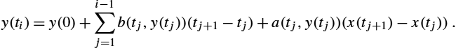
. The same distribution appears when we take the stochastic process view and use W in (10.18). We now take this to the manifold situation by starting the process (10.20) at a point u=(m,W)![]() in the frame bundle. This is a direct generalization of (10.18). When W is an orthonormal basis, the generated distribution is the transition distribution of a Riemannian Brownian motion. However, when W is not orthonormal, the generated distribution becomes anisotropic. Fig. 10.6 shows density plots of the Riemannian normal distribution and a Brownian motion both with W=0.5Idd
in the frame bundle. This is a direct generalization of (10.18). When W is an orthonormal basis, the generated distribution is the transition distribution of a Riemannian Brownian motion. However, when W is not orthonormal, the generated distribution becomes anisotropic. Fig. 10.6 shows density plots of the Riemannian normal distribution and a Brownian motion both with W=0.5Idd![]() , and an anisotropic distribution with W∝̸Idd
, and an anisotropic distribution with W∝̸Idd![]() .
.
 .
.We can write up the likelihood of observing a point y∈M![]() at time t=T
at time t=T![]() under the model,
under the model,
L(m,W;y)=p(T,y;m,W),
where p(t,y;m,W)![]() is the time t-density at the point y∈M
is the time t-density at the point y∈M![]() of the generated anisotropic distribution y(t)
of the generated anisotropic distribution y(t)![]() . Without loss of generality, the observation time can be set to T=1
. Without loss of generality, the observation time can be set to T=1![]() and skipped from the notation. The density can only be written with respect to a base measure, here denoted μ0
and skipped from the notation. The density can only be written with respect to a base measure, here denoted μ0![]() , such that y(T)=p(T;m,W)μ0
, such that y(T)=p(T;m,W)μ0![]() . If M
. If M![]() is Riemannian, then we can set μ0=dVg
is Riemannian, then we can set μ0=dVg![]() , but this is not a requirement: The construction only needs a connection and a fixed base measure with respect to which we define the likelihood.
, but this is not a requirement: The construction only needs a connection and a fixed base measure with respect to which we define the likelihood.
The parameters of the model, m and W, are represented by one element u of the frame bundle FM![]() , that is, the starting point of the process u(t)
, that is, the starting point of the process u(t)![]() in FM
in FM![]() . Writing θ for the parameters combined, we have θ=u=(m,W)
. Writing θ for the parameters combined, we have θ=u=(m,W)![]() . These parameters correspond to the mean m and covariance Σ=WWT
. These parameters correspond to the mean m and covariance Σ=WWT![]() for the Euclidean normal distribution N(m,Σ)
for the Euclidean normal distribution N(m,Σ)![]() . We can take a step further and define the mean for such a distribution to be x as we pursue below. Similarly, we can define the notion of infinitesimal square root covariance of y(T)
. We can take a step further and define the mean for such a distribution to be x as we pursue below. Similarly, we can define the notion of infinitesimal square root covariance of y(T)![]() to be W.
to be W.
10.5.2 Isotropic noise
The linear model (10.3) includes both the matrix W and isotropic noise ϵ∼N(0,σ2I)![]() . We now discuss how this additive structure can be modeled, including the case where W is not of full rank d.
. We now discuss how this additive structure can be modeled, including the case where W is not of full rank d.
We have so far considered distributions resulting from a Brownian motion analogues of isotropic normal distributions and seen that they can be represented by the frame bundle SDE (10.20). The fundamental structure is that u0![]() being orthonormal spreads the infinitesimal variation equally in all directions as seen by the Riemannian metric. There exists a subbundle of FM
being orthonormal spreads the infinitesimal variation equally in all directions as seen by the Riemannian metric. There exists a subbundle of FM![]() called the orthonormal frame bundle OM
called the orthonormal frame bundle OM![]() that consists of only such orthonormal frames. Solutions to (10.20) will always stay in OM
that consists of only such orthonormal frames. Solutions to (10.20) will always stay in OM![]() if u0∈OM
if u0∈OM![]() . We here use the symbol R for elements of OM
. We here use the symbol R for elements of OM![]() to emphasize their pure rotation, not the scaling effect. We can model the added isotropic noise by modifying the SDE (10.20) to
to emphasize their pure rotation, not the scaling effect. We can model the added isotropic noise by modifying the SDE (10.20) to
dW(t)=Hi(W(t))∘dx(t)i+Hi(R(t))∘dϵ(t)i,dR(t)=hR(t)(π⁎(dW)),
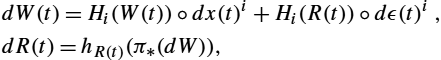
where the flow now has both the base point and covariance component W(t)![]() and a pure rotation R(t)
and a pure rotation R(t)![]() component serving as basis for the noise process ϵ(t)
component serving as basis for the noise process ϵ(t)![]() . As before, we let the generated distribution on M
. As before, we let the generated distribution on M![]() be y(t)=π(W(t))
be y(t)=π(W(t))![]() , that is, W(t)
, that is, W(t)![]() takes the place of u(t)
takes the place of u(t)![]() .
.
Elements of OM![]() differ only by a rotation, and since ϵ(t)
differ only by a rotation, and since ϵ(t)![]() is a Brownian motion scaled by σ, we can exchange R(t)
is a Brownian motion scaled by σ, we can exchange R(t)![]() in the right-hand side of dW(t)
in the right-hand side of dW(t)![]() by any other element of OM
by any other element of OM![]() without changing the distribution. Computationally, we can therefore skip R(t)
without changing the distribution. Computationally, we can therefore skip R(t)![]() from the integration and instead find an arbitrary element of OM
from the integration and instead find an arbitrary element of OM![]() at each time step of a numerical integration. This is particularly important when the dimension d of the manifold is large because R(t)
at each time step of a numerical integration. This is particularly important when the dimension d of the manifold is large because R(t)![]() has d2
has d2![]() components.
components.
We can explore this even further by letting W be a d×r![]() matrix with r≪d
matrix with r≪d![]() , thus reducing the rank of W similar to the PPCA situation (10.6). Without addition of the isotropic noise, this would in general result in the density p(⋅;m,W)
, thus reducing the rank of W similar to the PPCA situation (10.6). Without addition of the isotropic noise, this would in general result in the density p(⋅;m,W)![]() being degenerate, just as the Euclidean normal density function requires full rank covariance matrix. However, with the addition of the isotropic noise, W+σR
being degenerate, just as the Euclidean normal density function requires full rank covariance matrix. However, with the addition of the isotropic noise, W+σR![]() can still be of full rank even though W has zero eigenvalues. This has further computational advantages: If we instead of using the frame bundle FM
can still be of full rank even though W has zero eigenvalues. This has further computational advantages: If we instead of using the frame bundle FM![]() , let W be an element of the bundle of rank r linear maps Rr→TM
, let W be an element of the bundle of rank r linear maps Rr→TM![]() so that W1,…,Wr
so that W1,…,Wr![]() are r linearly independent basis vectors in Tπ(W)M
are r linearly independent basis vectors in Tπ(W)M![]() , and if we remove R(t)
, and if we remove R(t)![]() from the flow (10.22) as described before, then the flow now lives in a (d+rd)
from the flow (10.22) as described before, then the flow now lives in a (d+rd)![]() -dimensional fiber bundle compared to the d+d2
-dimensional fiber bundle compared to the d+d2![]() dimensions of the full frame bundle. For low r, this can imply a substantial reduction in computation time.
dimensions of the full frame bundle. For low r, this can imply a substantial reduction in computation time.
10.5.3 Euclideanization
Tangent space linearizations using the Expm![]() and Logm
and Logm![]() maps provide a linear view of the data yi
maps provide a linear view of the data yi![]() on M
on M![]() . When the data are concentrated close to a mean m, this view gives a good picture of the data variation. However, as data spread grows larger, curvature starts having an influence, and the linear view can provide a progressively distorted picture of the data. Whereas linear views of a curved geometry will never give truly faithful picture of the data, we can use a generalization of (10.3) to provide a linearization that integrates the effect of curvature at points far from m. The standard PCA dimension-reduced view of the data is writing W=UΛ
. When the data are concentrated close to a mean m, this view gives a good picture of the data variation. However, as data spread grows larger, curvature starts having an influence, and the linear view can provide a progressively distorted picture of the data. Whereas linear views of a curved geometry will never give truly faithful picture of the data, we can use a generalization of (10.3) to provide a linearization that integrates the effect of curvature at points far from m. The standard PCA dimension-reduced view of the data is writing W=UΛ![]() , where Λ is the diagonal matrix with the eigenvalues λ1,…,λr
, where Λ is the diagonal matrix with the eigenvalues λ1,…,λr![]() of W in the diagonal. In PPCA this is used to provide a low-dimensional representation of the data from the data conditional expectation x|yi
of W in the diagonal. In PPCA this is used to provide a low-dimensional representation of the data from the data conditional expectation x|yi![]() . This can be further reduced to a single data descriptor xi:=E[x|yi]
. This can be further reduced to a single data descriptor xi:=E[x|yi]![]() by taking expectation, and then we obtain an equivalent of the standard PCA view by displaying Λxi
by taking expectation, and then we obtain an equivalent of the standard PCA view by displaying Λxi![]() .
.
In the current probabilistic model, we can likewise condition the latent variables on the data to get a Euclidean entity describing the data. Since the latent variable is now a time-dependent path, the result of the conditioning is a process x(t)|y(T)=yi![]() where the conditioning is on the response process hitting the data at time T. This results in a quite different view of the data as illustrated in Fig. 10.7 and exemplified in Fig. 10.1: as in PPCA, taking expectation, we get
where the conditioning is on the response process hitting the data at time T. This results in a quite different view of the data as illustrated in Fig. 10.7 and exemplified in Fig. 10.1: as in PPCA, taking expectation, we get
ˉx(t)i=E[x(t)|y(T)=yi].
To get a single data descriptor, we can integrate dˉx(t)i![]() in time to get the endpoint xi:=∫T0dˉx(t)idt=ˉx(T)i
in time to get the endpoint xi:=∫T0dˉx(t)idt=ˉx(T)i![]() . From the example in Fig. 10.1 we see that this Euclideanization of the data can be quite different compared to tangent space linearization.
. From the example in Fig. 10.1 we see that this Euclideanization of the data can be quite different compared to tangent space linearization.
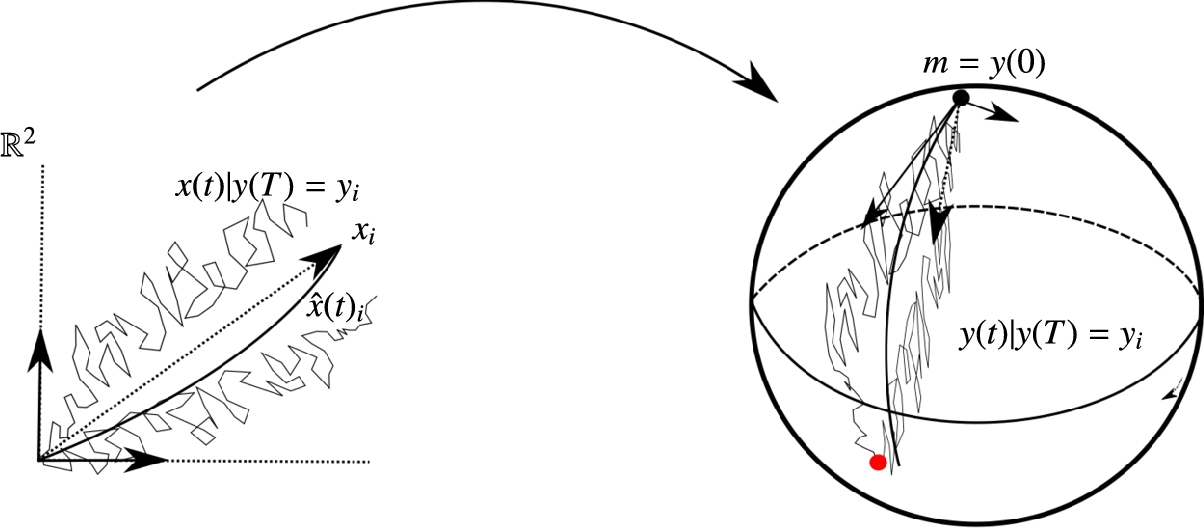 (this will generally only happen if M is Euclidean). The Euclidean process can be summarized into the expected path ˉx(t)i
 (thick curve left). This path can again be summarized by its endpoint xi, which is a single vector (dashed arrow left). Contrary to tangent space linearizations, the fact that the process visits all points of the manifold integrates curvature into this vector. It is thus not equivalent to Logm(yi).
10.6 Statistics with bundles
We now use the generalization of (10.3) via processes, either in the Lie algebra (10.17) of a group or on the frame bundle (10.20), to do statistics of manifold data. We start with ML estimation of mean and infinitesimal covariance by fitting anisotropic normal distributions to data, then progress to describing probabilistic PCA, a regression model, and estimation schemes.
10.6.1 Normal distributions and maximum likelihood
Considering the transition distribution μ(θ)=y(T)![]() of solutions u(t)
of solutions u(t)![]() to (10.20) projected to the manifold y(t)=π(u(t))
to (10.20) projected to the manifold y(t)=π(u(t))![]() started at θ=u=(m,W)
started at θ=u=(m,W)![]() a normal distribution with infinitesimal covariance Σ=WWT
a normal distribution with infinitesimal covariance Σ=WWT![]() , we can now define the sample maximum likelihood mean ˆmML
, we can now define the sample maximum likelihood mean ˆmML![]() by
by
ˆmML=argmaxmN∏i=1L(m;yi)

from samples y1,…,yN∈M![]() . Here, we implicitly assume that W is orthonormal with respect to a Riemannian metric. Alternatively, we can set
. Here, we implicitly assume that W is orthonormal with respect to a Riemannian metric. Alternatively, we can set
ˆmML=argmaxmmaxWN∏i=1L(m,W;yi),

where we simultaneously optimize to find the most likely infinitesimal covariance. The former definition defines ˆmML![]() as the starting point of the Brownian motion with transition density making the observations most likely. The latter includes the effect of the covariance, the anisotropy, and because of this it will in general give different results. In practice the likelihood is evaluated by Monte Carlo sampling. Parameter estimation procedures with parameters θ=(m)
as the starting point of the Brownian motion with transition density making the observations most likely. The latter includes the effect of the covariance, the anisotropy, and because of this it will in general give different results. In practice the likelihood is evaluated by Monte Carlo sampling. Parameter estimation procedures with parameters θ=(m)![]() or θ=(m,W)
or θ=(m,W)![]() and sampling methods are the topic of section 10.7.
and sampling methods are the topic of section 10.7.
We can use the likelihood (10.21) to get ML estimates for both the mean x and the infinitesimal covariance W by modifying (10.25) to
(ˆmML,ˆWML)=ˆuML=argmaxuN∏i=1L(u;yi).

Note the nonuniqueness of the result when estimating the square root W instead of the covariance Σ=WWT![]() . We discuss this point from a more geometric view in section 10.8.4.
. We discuss this point from a more geometric view in section 10.8.4.
10.6.2 Infinitesimal PPCA
The latent model (10.22) is used as the basis for the infinitesimal version of manifold PPCA [34], which we discussed in general terms in section 10.2.3. As in Euclidean PPCA, r denotes the number of principal eigenvectors to be estimated. With a fixed base measure μ0![]() , we write the density of the distribution generated from the low-rank plus noise system (10.22) as μ(m,W,σ)=p(T;m,W,σ)dVg
, we write the density of the distribution generated from the low-rank plus noise system (10.22) as μ(m,W,σ)=p(T;m,W,σ)dVg![]() and use this to define the likelihood L(m,W,σ;y)
and use this to define the likelihood L(m,W,σ;y)![]() in (10.12). The major difference in relation to (10.26) is now that the noise parameter σ is estimated from the data and that W is of rank r≤d
in (10.12). The major difference in relation to (10.26) is now that the noise parameter σ is estimated from the data and that W is of rank r≤d![]() .
.
The Euclideanization approach of section 10.5.3 gives equivalents of Euclidean principal components by conditioning the latent process on the data xi:=x(t)|y(T)=yi![]() . By taking expectation this can be reduced to a single path ˉx(t)i:=E[x(t)|y(T)=yi]
. By taking expectation this can be reduced to a single path ˉx(t)i:=E[x(t)|y(T)=yi]![]() or a single vector xi:=ˉx(T)i
or a single vector xi:=ˉx(T)i![]() .
.
The model is quite different from constructions of manifold PCA [11,14,31,5,27] that seek subspaces of the manifold having properties related to Euclidean linear subspaces. The probabilistic model and the horizontal frame bundle flows in general imply that no subspace is constructed in the present model. Instead, we can extract the parameters of the generated distribution and the information present in the conditioned latent process. As we discuss in section 10.8.1, the fact that the model does not generate subspaces is fundamentally linked to curvature, the curvature tensor, and nonintegrability of the horizontal distribution in FM![]() .
.
10.6.3 Regression
The generalized latent model (10.3) is used in [17] to define a related regression model. Here we assume observations (xi,yi)![]() , i=1,…,N
, i=1,…,N![]() , with xi∈Rd
, with xi∈Rd![]() and yi∈M
and yi∈M![]() . As in the previous models, the unknown is the point m∈M
. As in the previous models, the unknown is the point m∈M![]() , which takes the role of the intercept in multivariate regression, the coefficient matrix W, and the noise variance σ2
, which takes the role of the intercept in multivariate regression, the coefficient matrix W, and the noise variance σ2![]() . Whereas the infinitesimal nature of the model that relies on the latent variable being a semimartingale makes it geometrically natural, the fact that the latent variable is a process implies that its values in the interval (0,T)
. Whereas the infinitesimal nature of the model that relies on the latent variable being a semimartingale makes it geometrically natural, the fact that the latent variable is a process implies that its values in the interval (0,T)![]() are unobserved if xi
are unobserved if xi![]() is the observation at time T. This turns the construction into a missing data problem, and the values of x(t)
is the observation at time T. This turns the construction into a missing data problem, and the values of x(t)![]() in the unobserved interval (0,T)
in the unobserved interval (0,T)![]() needs to be integrated out. This can be pursued by combining bridge sampling as described below with matching of the sample moments of data with moments of the response variable y defined by the model [18].
needs to be integrated out. This can be pursued by combining bridge sampling as described below with matching of the sample moments of data with moments of the response variable y defined by the model [18].
10.7 Parameter estimation
So far we have only constructed models and defined parameter estimation as optimization problems for the involved likelihoods. It remains to discuss how we can actually estimate parameters in concrete settings. We describe here three approaches: (1) using a least-squares principle that incorporates the data anisotropy; this model is geometrically intuitive, but it only approximates the true density in the limit as T→0![]() . (2) Using the method of moments where approximations of low-order moments of the generated distribution is compared with the corresponding data moments. (3) Using bridge sampling of the conditioned process to approximate transition density functions with Monte Carlo sampling.
. (2) Using the method of moments where approximations of low-order moments of the generated distribution is compared with the corresponding data moments. (3) Using bridge sampling of the conditioned process to approximate transition density functions with Monte Carlo sampling.
10.7.1 Anisotropic least squares
The Fréchet mean (see Chapter 2) is defined from the least-squares principle. Here we aim to derive a similar least-squares condition for the variables θ=m![]() , θ=(m,W)
, θ=(m,W)![]() , or θ=(m,W,σ)
, or θ=(m,W,σ)![]() . With this approach, the inferred parameters ˆθ
. With this approach, the inferred parameters ˆθ![]() will only approximate the actual maximum likelihood estimates in a certain limit. Although only providing an approximation, the least-squares approach is different from Riemannian least-squares, and it is thereby both of geometric interest and gives perspective on the bridge sampling described later.
will only approximate the actual maximum likelihood estimates in a certain limit. Although only providing an approximation, the least-squares approach is different from Riemannian least-squares, and it is thereby both of geometric interest and gives perspective on the bridge sampling described later.
Until now we have assumed the observation time T to be strictly positive or simply T=1![]() . If instead we let T→0
. If instead we let T→0![]() , then we can explore the short-time asymptotic limit of the generated density. Starting with the Brownian motion, the limit has been extensively studied in the literature. For the Euclidean normal density, we know that pN(m,TId)(y)=(2πT)−d2exp(−‖y−m‖22T)
, then we can explore the short-time asymptotic limit of the generated density. Starting with the Brownian motion, the limit has been extensively studied in the literature. For the Euclidean normal density, we know that pN(m,TId)(y)=(2πT)−d2exp(−‖y−m‖22T)![]() . In particular, the density obeys the limit limT→0TlogpN(m,TId)(y)=−12‖y−m‖2
. In particular, the density obeys the limit limT→0TlogpN(m,TId)(y)=−12‖y−m‖2![]() . The same limit occurs on complete Riemannian manifolds with dist(m,y)2
. The same limit occurs on complete Riemannian manifolds with dist(m,y)2![]() instead of the norm ‖y−m‖2
instead of the norm ‖y−m‖2![]() and when y is outside the cut locus C(m)
and when y is outside the cut locus C(m)![]() ; see, for example, [13]. Thus, minimizing the squared distance to data can be seen as equivalent to maximizing the density, and hence the likelihood, for short running times of the Brownian motion specified by small T.
; see, for example, [13]. Thus, minimizing the squared distance to data can be seen as equivalent to maximizing the density, and hence the likelihood, for short running times of the Brownian motion specified by small T.
It is shown in [35] that there exists a function dQ:FM×M→R![]() that, for each u∈FM
that, for each u∈FM![]() , incorporates the anisotropy modeled in u in a measurement of the closeness dQ(u,y)
, incorporates the anisotropy modeled in u in a measurement of the closeness dQ(u,y)![]() of m=π(u)
of m=π(u)![]() and y. Like the Riemannian distance, which is defined as the minimal length or energy between curves linking two points in M
and y. Like the Riemannian distance, which is defined as the minimal length or energy between curves linking two points in M![]() , dQ
, dQ![]() is defined using curves in FM
is defined using curves in FM![]() from u to the fiber π−1(y)
from u to the fiber π−1(y)![]() over y but now with energy weighted by a matrix Σ−1
over y but now with energy weighted by a matrix Σ−1![]() :
:
dQ(u,y)=minu(t),u(0)=u,π(u(1))=y,˙u(t)∈HFM∫10˙u(t)TΣ−1(t)˙u(t)dt.

Here Σ(t)−1=(u(t)−1)Tu(t)−1![]() is the precision matrix of the infinitesimal covariance modeled in the frames u(t)
is the precision matrix of the infinitesimal covariance modeled in the frames u(t)![]() . The horizontality requirement ˙u(t)∈HFM
. The horizontality requirement ˙u(t)∈HFM![]() implies that the inner product defined by Σ(t)−1
implies that the inner product defined by Σ(t)−1![]() is parallel transported along with u(t)
is parallel transported along with u(t)![]() . The anisotropy is thus controlled by starting with a possibly nonorthonormal frame u0
. The anisotropy is thus controlled by starting with a possibly nonorthonormal frame u0![]() . We motivate this distance further from a geometric viewpoint in sections 10.8.2 and 10.8.3.
. We motivate this distance further from a geometric viewpoint in sections 10.8.2 and 10.8.3.
It is important here to relate the short-time T→0![]() asymptotic limit with the Euclidean normal density with covariance Σ. In the Euclidean case, the density is pN(m,TΣ)(y)=|2πTΣ|−12exp(−(y−m)TΣ−1(y−m)2T)
asymptotic limit with the Euclidean normal density with covariance Σ. In the Euclidean case, the density is pN(m,TΣ)(y)=|2πTΣ|−12exp(−(y−m)TΣ−1(y−m)2T)![]() and, as above, limT→0TlogpN(m,TΣ)(y)=−12(y−m)TΣ−1(y−m)
and, as above, limT→0TlogpN(m,TΣ)(y)=−12(y−m)TΣ−1(y−m)![]() . In the nonlinear situation using the Σ−1
. In the nonlinear situation using the Σ−1![]() weighted distance dQ
weighted distance dQ![]() , limT→0Tlogpμ(m,W)(y)=−12dQ(u,y)2
, limT→0Tlogpμ(m,W)(y)=−12dQ(u,y)2![]() . From this we can generalize the Fréchet mean least-squares principle to
. From this we can generalize the Fréchet mean least-squares principle to
ˆθ=(ˆm,ˆW)=argminu∈FMN∑i=1dQ(u,q−1(yi))2−N2log(detgu),
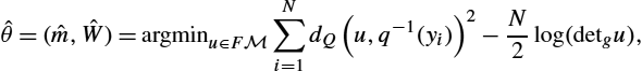
where log(detgu)![]() denotes the Riemannian determinant of the frame u. This term corresponds to the log-determinant in the Euclidean density pN(m,Σ)
denotes the Riemannian determinant of the frame u. This term corresponds to the log-determinant in the Euclidean density pN(m,Σ)![]() , and it acts to regularize the optimization that would otherwise increase W to infinity and reduce distances accordingly; ˆm
, and it acts to regularize the optimization that would otherwise increase W to infinity and reduce distances accordingly; ˆm![]() can be seen as an anisotropically weighted equivalent of the Fréchet mean.
can be seen as an anisotropically weighted equivalent of the Fréchet mean.
10.7.2 Method of moments
The method of moments compares low-order moments of the distribution with sample moments of the data. This can be used for parameter estimation by changing the parameters of the model to make the distribution and sample moments match as well as possible. The method of moments does not use the data likelihood, and it is dependent on ability to compute the moments in an appropriate space, for example, by embedding M![]() in a larger Euclidean space.
in a larger Euclidean space.
To compare first- and second-order moments, we can set up the cost function
S(μ(θ),〈y〉1,〈y〉2)=c1‖〈μ(θ)〉1−〈y〉1‖2+c2‖〈μ(θ)〉2−〈y〉2‖2,
where 〈μ(θ)〉1![]() and 〈y〉1
and 〈y〉1![]() denote the first-order moments of the distribution μ(θ)
denote the first-order moments of the distribution μ(θ)![]() and the sample moments of the data y1,…,yN
and the sample moments of the data y1,…,yN![]() , respectively, and similarly for the second-order moments 〈μ(θ)〉2
, respectively, and similarly for the second-order moments 〈μ(θ)〉2![]() and 〈y〉2
and 〈y〉2![]() , and c1,c2>0
, and c1,c2>0![]() are weights. If M
are weights. If M![]() is embedded in a larger Euclidean space, then the norms in (10.29) can be inherited from the embedding space norm. The optimal values of θ can then be found by minimizing this cost.
is embedded in a larger Euclidean space, then the norms in (10.29) can be inherited from the embedding space norm. The optimal values of θ can then be found by minimizing this cost.
This approach is used in [18] to estimate parameters in the regression model. The method of moments can be a computationally more lightweight alternative to the bridge sampling discussed further. In addition, the method can be a relatively stable approach because of the implicit regularization provided by only matching entities, here moments, that are averaged over the entire dataset. This is in contrast to the least-squares approach and the bridge sampling that estimate by evaluating dQ![]() or the likelihood on individual samples, and where averaging is done afterward, for example, by using averaged gradients when optimizing parameters. The moments 〈μ(θ)〉1
or the likelihood on individual samples, and where averaging is done afterward, for example, by using averaged gradients when optimizing parameters. The moments 〈μ(θ)〉1![]() and 〈μ(θ)〉2
and 〈μ(θ)〉2![]() can be approximated by sampling from the model or by approximation of the Fokker–Planck equation that governs the time evolution of the density; see, for example, [1].
can be approximated by sampling from the model or by approximation of the Fokker–Planck equation that governs the time evolution of the density; see, for example, [1].
10.7.3 Bridge sampling
At the heart of the methods discussed in this chapter are the data conditional latent processes x(t)|y(T)=yi![]() . We now describe methods for simulating from this conditioned process to subsequently approximate expectation of functions over the conditioned process and the transition density function.
. We now describe methods for simulating from this conditioned process to subsequently approximate expectation of functions over the conditioned process and the transition density function.
Stochastic bridges arise from conditioning a process to hit a point at a fixed time; here t=T![]() . Fig. 10.8 exemplifies the situation with samples from a Brownian bridge on S2
. Fig. 10.8 exemplifies the situation with samples from a Brownian bridge on S2![]() . Denoting the target point v, the expectation over the bridge process is related to the transition density p(T,v;m)
. Denoting the target point v, the expectation over the bridge process is related to the transition density p(T,v;m)![]() of the process by
of the process by
Ex(t)|x(T)=v[f(x(t))]=Ex(t)[f(x(t))1x(T)=v]p(T,v;m),

assuming that p(T,v;m)![]() is positive. Here 1 is the indicator function. Setting f(x(t))=1
is positive. Here 1 is the indicator function. Setting f(x(t))=1![]() , we can write this as
, we can write this as
p(T,v;m)=Ex(t)[1x(T)∈dv]dv
for an infinitesimal volume dv containing v. The transition density thus measures the combined probability mass of sample paths x(ω)(t)![]() with x(ω)(T)
with x(ω)(T)![]() near v. However, from the right-hand side of (10.31), we cannot directly get a good approach to computing the transition density and thereby the likelihood by sampling from x(t)
near v. However, from the right-hand side of (10.31), we cannot directly get a good approach to computing the transition density and thereby the likelihood by sampling from x(t)![]() because the probability of x(t)
because the probability of x(t)![]() hitting dv is arbitrarily small.
hitting dv is arbitrarily small.
 started at the north pole and conditioned on hitting a fixed point v∈S2
 (black point) at time T = 1.
Instead, we will use an approach to evaluate the conditional expectation Ex(t)|x(T)=v[f(x(t))]![]() by drawing samples from the bridge process and approximate the expectation by Monte Carlo sampling. We will see that this provides us with an effective way to evaluate the density p(T,v;m)
by drawing samples from the bridge process and approximate the expectation by Monte Carlo sampling. We will see that this provides us with an effective way to evaluate the density p(T,v;m)![]() . It is generally hard to simulate directly from the bridge process x(t)|x(T)=v
. It is generally hard to simulate directly from the bridge process x(t)|x(T)=v![]() . One exception is the Euclidean Brownian motion, where the bridge satisfies the SDE
. One exception is the Euclidean Brownian motion, where the bridge satisfies the SDE
dy(t)=−y(t)−vT−tdt+dW(t).
More generally, an arbitrary SDE (10.9) can be modified to give a bridge process by addition of an extra drift term:
dy(t)=b(t,y(t))dt+a(t,y(t))a(t,y(t))T∇logp(T−t,v;y(t))+a(t,y(t))dW(t).

This SDE could be used to simulate sample paths if it was not for the fact that it involves the gradient of the transition density p(T−t,v;y(t))![]() from the current value y(t)
from the current value y(t)![]() of the process to v. This transition density gradient generally does not have an explicit or directly computable form; indeed, our goal is to find a way to compute the transition density, and it is thus not feasible to use (10.33) computationally.
of the process to v. This transition density gradient generally does not have an explicit or directly computable form; indeed, our goal is to find a way to compute the transition density, and it is thus not feasible to use (10.33) computationally.
To improve on this situation, Delyon and Hu [4] proposed to use the added term from the Brownian bridge (10.32) instead of the gradient of the log-transition density giving an SDE of the form
dy(t)=b(t,y(t))dt−y(t)−vT−tdt+a(t,y(t))dW(t).
The drift term is illustrated in Fig. 10.9. Solutions y(t)![]() to (10.34) are not in general bridges of the original process. Instead, they are called guided processes. However, under certain conditions, the most important being that the diffusion field a is invertible, y(t)
to (10.34) are not in general bridges of the original process. Instead, they are called guided processes. However, under certain conditions, the most important being that the diffusion field a is invertible, y(t)![]() will hit v at time T a.s., and the law of the conditioned process x(t)|x(T)=v
will hit v at time T a.s., and the law of the conditioned process x(t)|x(T)=v![]() and the guided processes y(t)
and the guided processes y(t)![]() will be absolutely continuous with respect to each other with explicit Radon–Nikodym derivative φ. This implies that we can compute expectation over the bridge processes by taking the expectation of the guided process y(t)
will be absolutely continuous with respect to each other with explicit Radon–Nikodym derivative φ. This implies that we can compute expectation over the bridge processes by taking the expectation of the guided process y(t)![]() and correcting by factoring in φ:
and correcting by factoring in φ:
Ex(t)|x(T)=v[f(x(t))]=Ey(t)[f(y(t))φ(y(t))]Ey(t)[φ(y(t))].

Establishing this identity requires a nontrivial limiting argument to compare the two processes in the limit as t→T![]() , where the denominator T−t
, where the denominator T−t![]() in the guiding term in (10.34) approaches zero. As an additional consequence, Delyon and Hu and later Papaspiliopoulos and Roberts [28] write the transition density as the product of the Gaussian normal density and the expectation over the guided process of the correction factor:
in the guiding term in (10.34) approaches zero. As an additional consequence, Delyon and Hu and later Papaspiliopoulos and Roberts [28] write the transition density as the product of the Gaussian normal density and the expectation over the guided process of the correction factor:
p(T,v;m)=√|A(T,v)|(2πT)de−‖a(0,m)−1(m−v)‖22TEy(t)[φ(y(t))]

with A(t,x)=(a(t,x)−1)Ta(t,x)![]() . See also [36], where guided bridges are produced in a related way by using an approximation of the true transition density to replace p(T−t,v;y(t))
. See also [36], where guided bridges are produced in a related way by using an approximation of the true transition density to replace p(T−t,v;y(t))![]() in (10.33). The Delyon and Hu approach can be seen as a specific case of this where p(T−t,v;y(t))
in (10.33). The Delyon and Hu approach can be seen as a specific case of this where p(T−t,v;y(t))![]() is approximated by the transition density of a Brownian motion.
is approximated by the transition density of a Brownian motion.

 with the non-Euclidean landmark metric described in Chapter 4 and section 10.8.5.
10.7.4 Bridge sampling on manifolds
Extending the simulation scheme to general manifolds directly is nontrivial and the subject of ongoing research efforts. The fundamental issue is finding appropriate terms to take the role of the guiding term in (10.34) and controlling the behavior of such terms near the cut locus of the manifold. Here we instead sketch how the Delyon and Hu approach can be used in coordinates. This follows [30], where the approach is used for simulating from the Brownian motion on the landmark manifold described in chapter 4.
We assume that we have a chart covering the manifold up to a set of measure zero, and here we ignore the case where the stochastic process crosses this set. We take as an example the Riemannian Brownian motion with the coordinate process (10.15). Using the approach of Delyon and Hu, we get the guided processes
dy(t)=b(y(t))dt−y(t)−vT−tdt+√g(y(t))−1dB(t).
For the analysis in Delyon and Hu, we need the cometric g(y(t))−1![]() and its inverse, the metric g(y(t))
and its inverse, the metric g(y(t))![]() , to be bounded, whereas the drift coming from the Christoffel symbols can be unbounded or replaced by a bounded approximation. Then using (10.36), we get the expression
, to be bounded, whereas the drift coming from the Christoffel symbols can be unbounded or replaced by a bounded approximation. Then using (10.36), we get the expression
p(T,v;m)=√|g(v)|(2πT)de−(m−v)Tg(m)−1(m−v)2TEy(t)[φ(y)(t)].

This process is in coordinates and thus gives the density with respect to the Lebesgue measure on Rd![]() . We get the corresponding density with respect to dVg
. We get the corresponding density with respect to dVg![]() on M
on M![]() by removing the √|g(v)|
by removing the √|g(v)|![]() term:
term:
p(T,v;m)=(2πT)−d2e−(m−v)Tg(m)−1(m−v)2TEy(t)[φ(y)(t)].
The expectation Ey(t)[φ(y(t))]![]() has no closed-form expression in general. Instead, it can be approximated by Monte Carlo sampling by simulating processes (10.37) finitely many times and averaging the computed correction factors φ(y(t))
has no closed-form expression in general. Instead, it can be approximated by Monte Carlo sampling by simulating processes (10.37) finitely many times and averaging the computed correction factors φ(y(t))![]() .
.
With the machinery to approximate the likelihood in place, we can subsequently seek to optimize the likelihood with respect to the parameters θ. This can be done directly by computing the gradient with respect to θ of (10.38). This is a relatively complex expression to take derivatives of by hand. Instead, automatic differentiation methods can be used such as pursued in the Theano Geometry library, which we used to produce the examples in this chapter. This brings us to the following stochastic gradient descent algorithm for parameter estimation by bridge sampling, where we iteratively update the parameter estimate θl![]() :
:

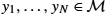 .
.10.8 Advanced concepts
Here we give more detail on some of the concepts that result from using a fiber bundle structure to model data variation on manifolds. In particular, we discuss how the Riemannian curvature tensor can be expressed directly as the vertical variation of frames resulting from the nonclosure of the bracket of horizontal vector fields. We then define a sub-Riemannian geometry on the frame bundle that has a notion of most probable paths as geodesics, and we discuss how to geometrically model the actual infinitesimal covariance matrix as compared to the square root covariance we have used so far. Finally, we give two examples of flows using special geometric structure, namely flows in the phase space of the landmark manifold.
Many of the concepts presented here are discussed in more detail in [35,33].
10.8.1 Curvature
The curvature of manifold is most often given in terms of the curvature tensor R∈T31(M)![]() , which is defined from the connection; see chapter 1. Let now u∈FM
, which is defined from the connection; see chapter 1. Let now u∈FM![]() be a frame considered as an element of GL(Rd,Tπ(u)M)
be a frame considered as an element of GL(Rd,Tπ(u)M)![]() . We use this identification between Tπ(u)M
. We use this identification between Tπ(u)M![]() and Rd
and Rd![]() to write the curvature form Ω:
to write the curvature form Ω:
Ω(vu,wu)=u−1R(π⁎(vu),π⁎(wu))u,vu,wv∈TFM.
Note that Ω takes values in gl(n)![]() : It describes how the identity map u−1u:Rd→Rd
: It describes how the identity map u−1u:Rd→Rd![]() changes when moving around an infinitesimal parallelogram determined by the tangent vectors π⁎(vu)
changes when moving around an infinitesimal parallelogram determined by the tangent vectors π⁎(vu)![]() and π⁎(wu)
and π⁎(wu)![]() with u kept fixed. It is thus vertical valued: It takes values in VFM. This can be made precise by employing an isomorphism ψ between FM×gl(n)
with u kept fixed. It is thus vertical valued: It takes values in VFM. This can be made precise by employing an isomorphism ψ between FM×gl(n)![]() and VFM given by ψ(u,v)=ddtuexp(tv)|t=0
and VFM given by ψ(u,v)=ddtuexp(tv)|t=0![]() using the Lie group exponential exp on GL(Rd)
using the Lie group exponential exp on GL(Rd)![]() ; see, for example, [19].
; see, for example, [19].
Now using the horizontal–vertical splitting of TFM![]() and ψ, we define a gl(n)
and ψ, we define a gl(n)![]() -valued vertical one-form ω:TFM→gl(n)
-valued vertical one-form ω:TFM→gl(n)![]() by
by
ω(vu)=0 if vu∈HFMω(vu)=ψ−1(vu) if vu∈VFM.

Here ω represents the connection via the horizontal–vertical splitting by singling out the vertical part of a TFM![]() vector and representing it as an element of gl(n)
vector and representing it as an element of gl(n)![]() [13]. Using ω, we have
[13]. Using ω, we have
ω([Hi,Hj])=−Ω(Hi,Hj),
and we see that the curvature form measures the vertical component of the bracket [Hi,Hj]=HiHj−HjHi![]() between horizontal vector fields. In other words, a nonzero curvature implies that the bracket between horizontal vector fields is nonzero.
between horizontal vector fields. In other words, a nonzero curvature implies that the bracket between horizontal vector fields is nonzero.
As a consequence, nonzero curvature implies that it is impossible to find a submanifold of FM![]() that has its tangent space being the span of the horizontal vector fields: For this to happen, the horizontal vector fields would need to present an integrable distribution by the Frobenius theorem, but the condition for this is exactly that the bracket between vector fields in this distribution must be closed. This is the reason why the infinitesimal PPCA model described here does not generate submanifolds of FM
that has its tangent space being the span of the horizontal vector fields: For this to happen, the horizontal vector fields would need to present an integrable distribution by the Frobenius theorem, but the condition for this is exactly that the bracket between vector fields in this distribution must be closed. This is the reason why the infinitesimal PPCA model described here does not generate submanifolds of FM![]() or M
or M![]() as in the Euclidean case.
as in the Euclidean case.
10.8.2 Sub-Riemannian geometry
A sub-Riemannian metric acts as a Riemannian metric except that it is not required to be strictly positive definite: It can have zero eigenvalues. We now define a certain sub-Riemannian metric on FM![]() that can be used to encode anisotropy and infinitesimal covariance. First, for u∈FM
that can be used to encode anisotropy and infinitesimal covariance. First, for u∈FM![]() , define the inner product Σ(u)
, define the inner product Σ(u)![]() on Tπ(u)M
on Tπ(u)M![]() by
by
Σ(u)−1(v,w)=〈u−1(v),u−1(w)〉Rd,v,w∈Tπ(u)M.
Note how u−1![]() maps the tangent vectors v, w to Rd
maps the tangent vectors v, w to Rd![]() before the standard Euclidean inner product is applied. To define an inner product on TFM
before the standard Euclidean inner product is applied. To define an inner product on TFM![]() , we need to connect this to tangent vectors in TFM
, we need to connect this to tangent vectors in TFM![]() . This is done using the pushforward of the projection π giving the inner product
. This is done using the pushforward of the projection π giving the inner product
gu(v,w)=Σ(u)−1(π⁎v,π⁎w).
This metric is quite different compared to a direct lift of a Riemannian metric to the frame bundle because of the application of u−1![]() in (10.41). This is a geometric equivalent of using the precision matrix Σ−1
in (10.41). This is a geometric equivalent of using the precision matrix Σ−1![]() as an inner product in the Gaussian density function. Here it is instead applied to infinitesimal displacements. Note that gu
as an inner product in the Gaussian density function. Here it is instead applied to infinitesimal displacements. Note that gu![]() vanishes on VFM
vanishes on VFM![]() because π⁎(v)=0
because π⁎(v)=0![]() for v∈VFM
for v∈VFM![]() . The inner product is therefore only positive definite on the horizontal subbundle HFM
. The inner product is therefore only positive definite on the horizontal subbundle HFM![]() .
.
For a curve u(t)∈FM![]() for which ˙u(t)∈HFM
for which ˙u(t)∈HFM![]() , we define the sub-Riemannian length of u(t)
, we define the sub-Riemannian length of u(t)![]() by
by
l(u(t))=∫10√gu(t)(˙u(t),˙u(t))dt.

If ˙u![]() is not a.e. horizontal, then we define l(u)=∞
is not a.e. horizontal, then we define l(u)=∞![]() ; l defines a sub-Riemannian distance, which is equivalent to the distance dQ
; l defines a sub-Riemannian distance, which is equivalent to the distance dQ![]() in section 10.7.1. Extremal curves are called sub-Riemannian geodesics. A subclass of these curves are the normal geodesics that can be computed from a geodesic equation as in the Riemannian case. Here we represent the sub-Riemannian metric as a map ˜g:TFM⁎→HFM⊆TFM
in section 10.7.1. Extremal curves are called sub-Riemannian geodesics. A subclass of these curves are the normal geodesics that can be computed from a geodesic equation as in the Riemannian case. Here we represent the sub-Riemannian metric as a map ˜g:TFM⁎→HFM⊆TFM![]() defined by gu(w,˜g(ξ))=(ξ|w)
defined by gu(w,˜g(ξ))=(ξ|w)![]() , ∀w∈HuFM
, ∀w∈HuFM![]() , ξ∈TFM⁎
, ξ∈TFM⁎![]() and define the Hamiltonian
and define the Hamiltonian
H(u,ξ)=12ξ(˜gu(ξ)).
In canonical coordinates the evolution of normal geodesics is then governed by the Hamiltonian system
˙ui=∂H∂ξi(u,ξ),˙ξi=−∂H∂ui(u,ξ)
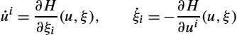
10.8.3 Most probable paths
The concept of path probability and maximizing path probability needs careful definitions because of the fact that sample paths of semimartingales are a.s. nowhere differentiable. It is therefore not possible to directly write up an energy for such paths using derivatives and to maximize such an energy. Instead, Onsager and Machlup [8] defined a notion of path-probability as the limit of progressively smaller tubes around smooth paths γ. Here we let μMϵ(γ)![]() be the probability that a process x(t)
be the probability that a process x(t)![]() stays within distance ϵ from the curve γ, that is,
stays within distance ϵ from the curve γ, that is,
μMϵ(γ)=P(dist(x(t),γ(t))<ϵ,∀t∈[0,1]).
The most probable path is the path that maximizes μϵM(γ)![]() as ϵ→0
as ϵ→0![]() .
.
For a Riemannian Brownian motion, Onsager and Machlup showed that
μMϵ(γ)∝exp(cϵ2+∫10LM(γ(t),˙γ(t))dt)

as ϵ→0![]() , where LM
, where LM![]() is the Onsager–Machlup functional
is the Onsager–Machlup functional
LM(γ(t),˙γ(t))=−12‖˙γ(t)‖2g+112Sg(γ(t)),
where Sg![]() is the scalar curvature. Notice the resemblance with the usual Riemannian energy except for the added scalar curvature term. Intuitively, this term senses the curvature of the manifold as the radii of the tubes around γ approaches zero.
is the scalar curvature. Notice the resemblance with the usual Riemannian energy except for the added scalar curvature term. Intuitively, this term senses the curvature of the manifold as the radii of the tubes around γ approaches zero.
Turning to the mapping of Euclidean processes to the manifold via the frame bundle construction, [32,35,33] propose to define the path probability of a process y(t)![]() on M
on M![]() that is a stochastic development of a Brownian motion x(t)
that is a stochastic development of a Brownian motion x(t)![]() on Rd
on Rd![]() by applying the Onsager–Machlup functional to the processes x(t)
by applying the Onsager–Machlup functional to the processes x(t)![]() . The path probability is thus measured in the Euclidean space. Extremal paths in this construction are called the most probable paths for the driving semimartingale, which in this case is x(t)
. The path probability is thus measured in the Euclidean space. Extremal paths in this construction are called the most probable paths for the driving semimartingale, which in this case is x(t)![]() . Because the scalar curvature term of LM
. Because the scalar curvature term of LM![]() is zero in the Euclidean space, we identify the curves as
is zero in the Euclidean space, we identify the curves as
argminy(t),y(0)=m,y(1)=y∫10−LRn(x(t),ddtx(t))dt.

The function turns out to be exactly the sub- Riemannian length defined in the previous section, and the most probable paths for the driving semimartingale therefore equal geodesics for the sub-Riemannian metric gu![]() . In particular, Hamiltonian equations (10.42) characterize the subclass of normal geodesics. Fig. 10.10 illustrates such curves, which are now extremal for the anisotropically weighted metric.
. In particular, Hamiltonian equations (10.42) characterize the subclass of normal geodesics. Fig. 10.10 illustrates such curves, which are now extremal for the anisotropically weighted metric.
 from the north pole (red dot (dark gray in print version)) to a point on the southern hemisphere (blue dot (light gray in print version)). Left: isotropic process; center and right: processes with covariance visualized by the frame (arrows) at the north pole and the ellipses. The parallel transport of the frame along the most probable paths is plotted. The sphere is colored by an approximation of the generated transition density. It can be clearly seen how increasing anisotropy interacts with curvature to give most probable paths that are not aligned with geodesics. Intuitively, the most probable paths tend to stay in high-density areas on the northern hemisphere before taking the “shorter” low-probability route to the target point on the southern hemisphere.
10.8.4 Bundles without rotation
When modeling infinitesimal covariance, the frame bundle in a sense provides an overspecification because u∈FM![]() represents square root covariances √Σ
represents square root covariances √Σ![]() and not Σ directly. Multiple such square roots can represent the same Σ. To remedy this, we can factorize the inner product Σ−1(u)
and not Σ directly. Multiple such square roots can represent the same Σ. To remedy this, we can factorize the inner product Σ−1(u)![]() above through the bundle Sym+
above through the bundle Sym+![]() of symmetric positive definite covariant 2-tensors on M
of symmetric positive definite covariant 2-tensors on M![]() . We have
. We have
FMΣ−1→Sym+Mq→M,
and Σ−1(u)![]() can now directly be seen as an element of Sym+
can now directly be seen as an element of Sym+![]() . The polar decomposition theorem states that Sym+
. The polar decomposition theorem states that Sym+![]() is isomorphic to the quotient FM/O(Rd)
is isomorphic to the quotient FM/O(Rd)![]() with O(Rd)
with O(Rd)![]() being orthogonal transformations on Rd
being orthogonal transformations on Rd![]() . The construction thus removes the rotation from FM
. The construction thus removes the rotation from FM![]() that was the over-specification representing the square root covariance. The fiber bundle structure and horizontality that we used on FM
that was the over-specification representing the square root covariance. The fiber bundle structure and horizontality that we used on FM![]() descend to Sym+
descend to Sym+![]() . In practice we can work on Sym+
. In practice we can work on Sym+![]() and FM
and FM![]() interchangeably. It is often more direct to write SDEs and stochastic development on FM
interchangeably. It is often more direct to write SDEs and stochastic development on FM![]() , which is why we generally prefer this instead of using Sym+
, which is why we generally prefer this instead of using Sym+![]() .
.
10.8.5 Flows with special structure
We have so far created parametric families of probability distribution on general manifold using stochastic processes, either the Brownian motion or stochastic developments of Euclidean semimartingales. Here we briefly mention other types of processes that use special structure of the underlying space and that can be used to construct distributions for performing parameter estimation. We focus on three cases of flows of the LDDMM landmark manifold discussed in chapter 4.
The landmark geodesic equations with the metric discussed in Chapter 4 are usually written in the Hamiltonian form
˙qi=∂H∂pi(q,p),˙pi=−∂H∂qi(q,p),

with the position coordinates q=(q1,…,qn)![]() of the n landmarks, the momentum coordinates p, and the Hamiltonian H(q,p)=pTK(q,q)p
of the n landmarks, the momentum coordinates p, and the Hamiltonian H(q,p)=pTK(q,q)p![]() . We can use this phase-space formulation to introduce noise that is coupled to the momentum variable instead of only affecting the position equation, q, as pursued so far.
. We can use this phase-space formulation to introduce noise that is coupled to the momentum variable instead of only affecting the position equation, q, as pursued so far.
A construction for this is given by Trouvé and Vialard [38] by adding noise in the momentum variable with position and momentum dependent infinitesimal covariance
dqi=∂H∂pi(q,p),dpi=−∂H∂qi(q,p)dt+ϵi(q,p)dx(t),

where x(t)![]() is a Brownian motion on Rnd
is a Brownian motion on Rnd![]() . Similarly, Marsland and Shardlow define the stochastic Langevin equations
. Similarly, Marsland and Shardlow define the stochastic Langevin equations
dqi=∂H∂pi(q,p),dpi=−λ∂H∂qi(q,p)−∂H∂qi(q,p)dt+ϵdxi(t).

In both cases the noise directly affects the momentum.
A related but somewhat different model is the stochastic EPDiff equation by Arnaudon et al. [1]. Here a family of fields σ1,…,σJ![]() is defined on the domain Ω where the landmark reside, and noise is multiplied on these fields:
is defined on the domain Ω where the landmark reside, and noise is multiplied on these fields:
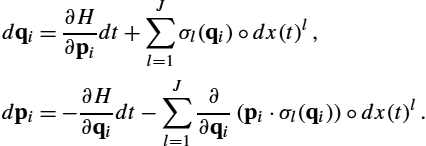
Here the driving Brownian motion ![]() is
is ![]() -valued. Notice the coupling to the momentum equation by the derivative of the noise fields. The stochasticity is in a certain sense compatible with the geometric construction that is used to define the LDDMM landmark metric. In particular, the momentum map construction [2] is preserved, and the landmarks equations are extremal for a stochastic variational principle
-valued. Notice the coupling to the momentum equation by the derivative of the noise fields. The stochasticity is in a certain sense compatible with the geometric construction that is used to define the LDDMM landmark metric. In particular, the momentum map construction [2] is preserved, and the landmarks equations are extremal for a stochastic variational principle
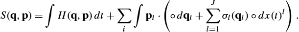
Bridge sampling on these processes can be pursued with the Delyon and Hu approach, and this can again be used to infer parameters of the model. In this case, the parameter set includes parameters for the noise fields ![]() . However, the diffusion field is in this case in general not invertible as was required by the guidance scheme (10.34). This necessitates extra care when constructing the guiding process [1]. Bridge simulation for the Trouvé–Vialard and Marsland–Shardlow models (10.45) and (10.46) can be pursued with the simulation approach of Schauer and van der Meulen; see [3].
. However, the diffusion field is in this case in general not invertible as was required by the guidance scheme (10.34). This necessitates extra care when constructing the guiding process [1]. Bridge simulation for the Trouvé–Vialard and Marsland–Shardlow models (10.45) and (10.46) can be pursued with the simulation approach of Schauer and van der Meulen; see [3].
In these examples, the Euclidean structure of the landmark domain Ω is used in defining the SDEs by using either the coordinates on the momentum variable in (10.45) and (10.46) or by using the noise fields ![]() on Ω in the stochastic EPDiff case (10.48). In the latter example, the construction is furthermore related to the representation of the landmark space as a homogeneous space arising from quotienting a subgroup of the diffeomorphism group
on Ω in the stochastic EPDiff case (10.48). In the latter example, the construction is furthermore related to the representation of the landmark space as a homogeneous space arising from quotienting a subgroup of the diffeomorphism group ![]() by the isotropy group of the landmarks. On this subgroup of
by the isotropy group of the landmarks. On this subgroup of ![]() , there exists an SDE driven by the right-invariant noise defined by
, there exists an SDE driven by the right-invariant noise defined by ![]() . Solutions of this SDE project to solutions of (10.47). A further interpretation of the fields
. Solutions of this SDE project to solutions of (10.47). A further interpretation of the fields ![]() is that they represent noise in Eulerian coordinates, and they thereby use the Eulerian coordinate frame for defining the infinitesimal covariance.
is that they represent noise in Eulerian coordinates, and they thereby use the Eulerian coordinate frame for defining the infinitesimal covariance.
In all cases the parameters θ can be estimated from observed landmark configurations ![]() by maximum likelihood. The parameters θ can specify the starting conditions
by maximum likelihood. The parameters θ can specify the starting conditions ![]() of the process, the shape and position of
of the process, the shape and position of ![]() , and even parameters for the Riemannian metric on the landmark space.
, and even parameters for the Riemannian metric on the landmark space.
10.9 Conclusion
The aim of the chapter is to provide examples of probabilistic approaches to manifold statistics and ways to construct parametric families of probability distributions in geometrically natural ways. We pursued this using transition distributions of several stochastic processes: the Riemannian Brownian motion, Brownian motion on Lie groups, anisotropic generalizations of the Brownian motion by use of stochastic development, and finally flows that use special structure related to the particular space, the shape space of landmarks. We have emphasized the role of infinitesimal covariance modeled by frames in tangent spaces when defining SDEs and stochastic processes. In the Lie group setting, left-invariant vector fields provided this basis. In the general situation, we lift to the frame bundle to allow use of the globally defined horizontal vector fields on ![]() .
.
As illustrated from the beginning of the chapter in Fig. 10.1, probabilistic approaches can behave quite differently from their least-squares counterparts. We emphasized the coupling between covariance and curvature both visually and theoretically, the latter with the link between curvature and nonclosedness of the horizontal distribution, sub-Riemannian geodesics, and most probable paths for the driving semimartingales.
Finally we used the geometric and probabilistic constructions to describe statistical concepts such as the maximum likelihood mean from the Brownian motion, and maximum likelihood mean and infinitesimal covariance, and we provided ways of optimizing the parameters using bridge sampling.
The theoretical development of geometric statistics is currently far from complete, and there are many promising directions to be explored to approach as complete a theory of geometric statistics as is available for linear statistics. The viewpoint of this chapter is that probabilistic approaches play an important role in achieving this.
10.10 Further reading
Here we provide a few useful example references for background information and further reading.
An introduction to general SDE theory can be found in [25]. Much of the frame bundle theory, stochastic analysis on manifolds using frame bundles, and theory of Brownian motion on manifolds can be found in [13]. See also [7] for details on stochastic analysis on manifolds. Brownian motion on Lie groups is, for example, covered in [20]. Diffusions on stratified spaces is described in the works [23,24] by Tom Nye.
The relation between the horizontal subbundle and curvature can be found in the book [19]. Sub-Riemannian geometry is covered extensively in [22]. The stochastic large deformation model in [1] builds on the stochastic variational method of Holm [12].