
Spatially adaptive metrics for diffeomorphic image matching in LDDMM
Laurent Rissera,c; François-Xavier Vialardb,c aInstitut de Mathématiques de Toulouse, CNRS, Université de Toulouse, UMR CNRS 5219, Toulouse, France
bLaboratoire d'informatique Gaspard Monge, Université Paris-Est Marne-la-Vallée, UMR CNRS 8049, Champs sur Marne, France
cBoth authors equally contributed to the chapter.
Abstract
Registering two medical images consists in computing a mapping between the organs of interest they contain. Although this mapping is dense in space, it can only be accurately estimated based on significant intensity variations in the images, which is a sparse information. Using deformation regularization properties that are physiologically meaningful is then one of the keys to estimate pertinent mappings. In the LDDMM framework these regularization properties are directly related to the right-invariant metric which controls the optimal deformation. In this chapter we then present different methodologies related to this degree of freedom. After briefly introducing the LDDMM framework, we present a simple strategy to regularize the mappings at different scales and a more advanced technique to make it possible to estimate a sliding motion at predefined locations. We then propose to switch the paradigm of right-invariant metrics to left-invariant ones, so that spatially adaptive metrics can be used in LDDMM. In the last part, we review different attempts to optimize these spatially adaptive metrics and propose a new evolution of LDDMM that incorporates spatially adaptive metrics.
Keywords
Large deformation diffeomorphic metric mapping (LDDMM); spatially adaptive metric; multiscale kernel; sliding motion constraints; left-invariant diffeomorphic metric (LIDM); semidirect product of groups
14.1 Introduction to LDDMM
14.1.1 Problem definition
The construction of the large deformation diffeomorphic metric mapping (LDDMM) framework is based on a variational setting and the choice of a Riemannian metric. Its goal is to estimate optimal smooth and invertible maps (diffeomorphisms) of the ambient space that represent a mapping between the points of a source image IS![]() and those of a target image IT
and those of a target image IT![]() [9,6], see also Chapter 4. This diffeomorphic image registration formalism is particularly adapted to the registration of most 3D medical images, where the hypothesis that organ deformations are smooth is reasonable, and the topology of the represented organs is preserved. Note that this second property is mainly due to the fact that there is no occlusion or out-of-slice motion in such images. Image registration thus takes the form of an infinite-dimensional optimal control problem: Minimize the cost functional
[9,6], see also Chapter 4. This diffeomorphic image registration formalism is particularly adapted to the registration of most 3D medical images, where the hypothesis that organ deformations are smooth is reasonable, and the topology of the represented organs is preserved. Note that this second property is mainly due to the fact that there is no occlusion or out-of-slice motion in such images. Image registration thus takes the form of an infinite-dimensional optimal control problem: Minimize the cost functional
J(ξ)=12∫10‖ξ(t)‖2Vdt+S(IS∘φ−1)
under the constraints
∂tφ(t,x)=ξ(t,φ(t,x)),
φ(0,x)=x ∀x∈D.
The functional S![]() represents the similarity measure between the registered images. For grey level images acquired using the same modality (e.g. a pair of MR images), the standard similarity metric is the so-called sum of squared differences between the deformed source image IS
represents the similarity measure between the registered images. For grey level images acquired using the same modality (e.g. a pair of MR images), the standard similarity metric is the so-called sum of squared differences between the deformed source image IS![]() and the target image IT
and the target image IT![]() , that is, ‖IS∘φ−1−IT‖2L2
, that is, ‖IS∘φ−1−IT‖2L2![]() , both defined on a domain of the Euclidean space denoted by D. As summarized in Fig. 14.1, constraints (14.2) encode the trajectory of the points x∈D
, both defined on a domain of the Euclidean space denoted by D. As summarized in Fig. 14.1, constraints (14.2) encode the trajectory of the points x∈D![]() : At time t=0
: At time t=0![]() a point x of the source image IS
a point x of the source image IS![]() is naturally at location φ(0,x)=x
is naturally at location φ(0,x)=x![]() . Then its motion at times t∈[0,1]
. Then its motion at times t∈[0,1]![]() is defined by the integration of the time-dependent velocity field ξ(t,x)
is defined by the integration of the time-dependent velocity field ξ(t,x)![]() . The transformed location of x at time t=1
. The transformed location of x at time t=1![]() is finally φ(1,x)
is finally φ(1,x)![]() and corresponds to the mapping of x in the target image IT
and corresponds to the mapping of x in the target image IT![]() .
.

14.1.2 Properties
In Eq. (14.1), V is a Hilbert space of vector fields on a Euclidean domain D⊂Rd![]() . A key technical assumption, which ensures that the computed maps are diffeomorphisms up to the numerical scheme accuracy, is that the inclusion map V↪W1,∞(D,Rd)
. A key technical assumption, which ensures that the computed maps are diffeomorphisms up to the numerical scheme accuracy, is that the inclusion map V↪W1,∞(D,Rd)![]() , that is, the space of vector fields which are Lipschitz continuous, is continuous. The norm on V controls the W1,∞
, that is, the space of vector fields which are Lipschitz continuous, is continuous. The norm on V controls the W1,∞![]() norm, and we call such a space V an admissible space of vector fields. In particular, these spaces are included in the family of reproducing kernel Hilbert spaces (RKHS) [3] since pointwise evaluations are a continuous linear map, which implies that such spaces are completely defined by their kernel. The kernel, denoted by k
norm, and we call such a space V an admissible space of vector fields. In particular, these spaces are included in the family of reproducing kernel Hilbert spaces (RKHS) [3] since pointwise evaluations are a continuous linear map, which implies that such spaces are completely defined by their kernel. The kernel, denoted by k![]() in this chapter, is a function from the product space D×D
in this chapter, is a function from the product space D×D![]() into Rd
into Rd![]() that automatically satisfies the technical assumption mentioned if it is sufficiently smooth. Last, we denote by K:V⁎→V
that automatically satisfies the technical assumption mentioned if it is sufficiently smooth. Last, we denote by K:V⁎→V![]() the isomorphism between V⁎
the isomorphism between V⁎![]() , the dual of V, and V.
, the dual of V, and V.
Note that the contributions presented in this chapter build on the flexibility of the RKHS construction not only to accurately match the structure boundaries in the deformed source image IS∘φ−1![]() and the target image IT
and the target image IT![]() , but also to estimate physiologically plausible final deformation maps φ.
, but also to estimate physiologically plausible final deformation maps φ.
The direct consequence of the admissible hypothesis on V is that the flow of a time-dependent vector field in L2([0,1],V)![]() is well defined; see [29, Appendix C]. Then the set of flows at time 1 defines a group of diffeomorphisms denoted by GV
is well defined; see [29, Appendix C]. Then the set of flows at time 1 defines a group of diffeomorphisms denoted by GV![]() ; that is, denoting
; that is, denoting
Fl1(ξ)=φ(1) where φ solves (14.2),
define
GVdef.={φ(1):∃ξ∈L2([0,1],V) s.t. Fl1(ξ)},
which has been introduced by Trouvé [25]. On this group, Trouvé defines the metric
dist(ψ1,ψ0)2=inf{∫10‖ξ‖2Vdt:ξ∈L2([0,1],V) s.t. ψ1=Fl1(ξ)∘ψ0},
under which he proves that GV![]() is complete. In full generality very few mathematical properties of this group are known. However, in particular situations, such as where the space V is the space of Sobolev vector fields that satisfy the continuous injection property, then the group is also an infinite-dimensional Riemannian manifold (see [8]). Since the distance (14.6) is right-invariant, it is important to emphasize that for all ψ1,ψ2,ψ3∈GV
is complete. In full generality very few mathematical properties of this group are known. However, in particular situations, such as where the space V is the space of Sobolev vector fields that satisfy the continuous injection property, then the group is also an infinite-dimensional Riemannian manifold (see [8]). Since the distance (14.6) is right-invariant, it is important to emphasize that for all ψ1,ψ2,ψ3∈GV![]() , we have the following property:
, we have the following property:
dist(ψ1∘ψ3,ψ0∘ψ3)=dist(ψ1,ψ0).
Instead of formulating the variational problem on the group of diffeomorphisms GV![]() , it is often possible to rewrite the optimization problem on the space of images. More precisely, the minimization problem is taken to be
, it is often possible to rewrite the optimization problem on the space of images. More precisely, the minimization problem is taken to be
J(ξ)=∫10‖ξ(t)‖2Vdt+S(I(1))
under the constraints
∂tI(t,x)+〈∇I(t,x),ξ(t,x)〉=0,I(0,x)=IS(x) ∀x∈D.

For S(I(1))=ϵ1‖I(1)−IT‖2L2![]() , the sum of squared differences and σ is a positive parameter, and using the Lagrange multiplier rule, we can write the gradient of this functional as
, the sum of squared differences and σ is a positive parameter, and using the Lagrange multiplier rule, we can write the gradient of this functional as
∇J(ξ)=2ξ(t)+K(∇I(t)P(t)),
where P(t)![]() satisfies the continuity equation (the notation div stands for the divergence operator)
satisfies the continuity equation (the notation div stands for the divergence operator)
∂tP(t,x)+div(Pξ)=0
and the initial condition P(1)=2ϵ1(I(1)−IT)![]() . Therefore Eq. (14.10) has to be solved backward in time from t=1
. Therefore Eq. (14.10) has to be solved backward in time from t=1![]() to t=0
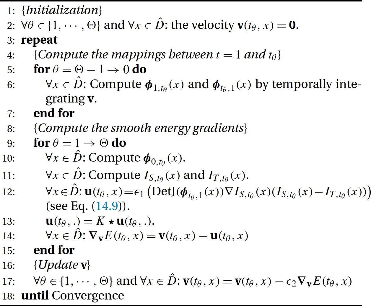
to t=0![]() . Alternatively, using the solutions of continuity and advection equations in terms of the flow map, it is possible to rewrite the gradient as in (line 12 of) Algorithm 14.1, which will be discussed in Section 14.1.3.
. Alternatively, using the solutions of continuity and advection equations in terms of the flow map, it is possible to rewrite the gradient as in (line 12 of) Algorithm 14.1, which will be discussed in Section 14.1.3.
More generally, it is possible to formulate the equivalent variational problem in the case where shapes are deformed rather than images, as, for instance, when registering point clouds or surfaces. Under mild conditions, it is also possible to prove that this approach induces a Riemannian metric on the orbit of the group action in some finite-dimensional cases (see also Chapter 4). We denote by Q the space of objects or shapes on which the deformation group is acting. When Q is an infinite-dimensional Riemannian manifold, the geometric picture is more complicated [5].
We now go back to the optimization problem. By first-order optimality and using again the notation J![]() for the corresponding but different functional, a solution to formulation (14.1) can be written as
for the corresponding but different functional, a solution to formulation (14.1) can be written as
J(P0)=12∫DK(P0∇I0)(x)P0(x)∇I0(x)dx+S(I(1))
under the constraints
{∂tI+〈∇I,ξ〉=0,∂tP+div(Pξ)=0,ξ+K(P0∇I0)(x)=0,
with initial conditions P(t=0)=P0![]() and I(t=0)=I0
and I(t=0)=I0![]() . The function P0:D↦R
. The function P0:D↦R![]() is sometimes called the momentum or scalar momentum, and we denoted
is sometimes called the momentum or scalar momentum, and we denoted
K(P0∇I0)(x)=∫Dk(x,y)P0(y)∇I0(y)dy;
in particular, this quantity can be reformulated as an L2![]() norm of the quantity P0∇I0
norm of the quantity P0∇I0![]() for the square root of the kernel k. Moreover, system (14.12) encodes the fact that the evolution of I(t)
for the square root of the kernel k. Moreover, system (14.12) encodes the fact that the evolution of I(t)![]() is geodesic in the LDDMM setting; see [28]. Therefore this formulation transforms the problem of optimizing on the time-dependent d-dimensional vector field ξ (sometimes called path-based optimization) into optimizing on a function P0
is geodesic in the LDDMM setting; see [28]. Therefore this formulation transforms the problem of optimizing on the time-dependent d-dimensional vector field ξ (sometimes called path-based optimization) into optimizing on a function P0![]() defined on the domain D (sometimes called shooting method). At optimality the following fixed point equation has to be satisfied:
defined on the domain D (sometimes called shooting method). At optimality the following fixed point equation has to be satisfied:
P(1)+∂IS(I(1))=0,
which can be used in practice for some optimization schemes [1].
14.1.3 Implementation
We now discuss different ideas related to the implementation of the LDDMM framework to register a source image IS![]() onto a target image IT
onto a target image IT![]() . Our discussion specifically builds on [6], where a practical algorithm of LDDMM for image matching was given. We then give hereafter an overview of this algorithm plus different numerical strategies we used to make it work efficiently. Note that our implementation of [6] and the extensions we developed are freely available on sourceforge.1
. Our discussion specifically builds on [6], where a practical algorithm of LDDMM for image matching was given. We then give hereafter an overview of this algorithm plus different numerical strategies we used to make it work efficiently. Note that our implementation of [6] and the extensions we developed are freely available on sourceforge.1
When registering two images, we have first to define a discrete domain on which φ(t,x)![]() and v(t,x)
and v(t,x)![]() are computed, where φ(t,x)
are computed, where φ(t,x)![]() is the mapping of x at time t through φ, and v(t,x)
is the mapping of x at time t through φ, and v(t,x)![]() is the velocity field integrated in time to compute φ. A natural choice is to use a spatial grid defined by the pixel/voxel coordinates of IS
is the velocity field integrated in time to compute φ. A natural choice is to use a spatial grid defined by the pixel/voxel coordinates of IS![]() . We denote by ˆD
. We denote by ˆD![]() this discrete domain and recall that D is the dense image domain. Linear interpolation is recommended to estimate φ and v at point locations in D and outside ˆD
this discrete domain and recall that D is the dense image domain. Linear interpolation is recommended to estimate φ and v at point locations in D and outside ˆD![]() . Note that IS
. Note that IS![]() and IT
and IT![]() may have a different resolution or may not be aligned. We suppose here that they have already been aligned by a rigid deformation and that the final deformation φ(1,x)
may have a different resolution or may not be aligned. We suppose here that they have already been aligned by a rigid deformation and that the final deformation φ(1,x)![]() is composed with this deformation to reach the pixel/voxel coordinates of IT
is composed with this deformation to reach the pixel/voxel coordinates of IT![]() . In our implementation we also used an uniformly sampled grid to discretize t. The grid time step should also be sufficiently small to avoid generating noninvertible deformations when temporally integrating v. About 10 time steps are enough in most applications, but more time steps may be necessary when sharp deformations are computed [18].
. In our implementation we also used an uniformly sampled grid to discretize t. The grid time step should also be sufficiently small to avoid generating noninvertible deformations when temporally integrating v. About 10 time steps are enough in most applications, but more time steps may be necessary when sharp deformations are computed [18].
We use the following notations to describe the registration algorithm: tθ,θ∈{1,…,Θ}![]() , are the discrete time points. For each tθ
, are the discrete time points. For each tθ![]() , several vector fields are required to encode useful deformations based on the diffeomorphism φ: ϕtj,ti(x)
, several vector fields are required to encode useful deformations based on the diffeomorphism φ: ϕtj,ti(x)![]() first transports x∈ˆD
first transports x∈ˆD![]() from time ti
from time ti![]() to time tj
to time tj![]() through φ. The images IS,tθ
through φ. The images IS,tθ![]() and IT,tθ
and IT,tθ![]() also correspond to IS
also correspond to IS![]() and IT
and IT![]() transported at time tθ
transported at time tθ![]() using ϕ0,tθ
using ϕ0,tθ![]() and ϕ1,tθ
and ϕ1,tθ![]() respectively. Image registration is then a gradient descent algorithm where v is optimized with respect to IS
respectively. Image registration is then a gradient descent algorithm where v is optimized with respect to IS![]() , IT
, IT![]() , and the smoothing kernel K as shown Algorithm 14.1.
, and the smoothing kernel K as shown Algorithm 14.1.
We can first remark that the mappings ϕ1,tθ(x)![]() and ϕtθ,1(x)
and ϕtθ,1(x)![]() are precomputed in the for loop at lines 5–7 of Algorithm 14.1. These mappings are indeed computed once for all and stored by using an Euler method from time tΘ
are precomputed in the for loop at lines 5–7 of Algorithm 14.1. These mappings are indeed computed once for all and stored by using an Euler method from time tΘ![]() to time t0
to time t0![]() , whereas the mappings ϕ0,tθ(x)
, whereas the mappings ϕ0,tθ(x)![]() can be computed from time t0
can be computed from time t0![]() to time tΘ
to time tΘ![]() in the energy gradients estimation loop.
in the energy gradients estimation loop.
We also strongly recommend to compute IS,tθ(x)![]() and IT,tθ(x)
and IT,tθ(x)![]() by resampling IS
by resampling IS![]() and IT
and IT![]() using ϕ0,tθ(x)
using ϕ0,tθ(x)![]() and ϕ1,tθ(x)
and ϕ1,tθ(x)![]() , respectively. An alternative would be to compute iteratively the deformed images time point after time point, for example, to compute IS,tθ(x)
, respectively. An alternative would be to compute iteratively the deformed images time point after time point, for example, to compute IS,tθ(x)![]() using IS,tθ−1(x)
using IS,tθ−1(x)![]() and v(tθ−1,x)
and v(tθ−1,x)![]() . This strategy would be far less memory consuming than the one we use, but it would also numerically diffuse the image intensities due to the iterative resamplings.
. This strategy would be far less memory consuming than the one we use, but it would also numerically diffuse the image intensities due to the iterative resamplings.
Another remark is that a simple and very efficient technique can be used to speed up the convergence of this registration algorithm. So-called momentum methods [15] are widely known in machine learning to speed up the convergence of gradient descent algorithms in high dimension. At each iteration it simply consists in updating the optimized variables with a linear combination of the current gradients and the previous update. Our (unpublished) experiences have shown that this technique is particularly efficient in image registration where, at a given iteration, the mapping can be already accurate in some regions and inaccurate in other regions.
The most important point to discuss to make the practical use of the LDDMM algorithm clear is that it depends on two parameters ϵ1![]() and ϵ2
and ϵ2![]() , respectively the weight in front of the sum of squared differences (see discussion for Eqs. (14.9) and (14.10)) and the step length of the gradient descent. In practice ϵ1
, respectively the weight in front of the sum of squared differences (see discussion for Eqs. (14.9) and (14.10)) and the step length of the gradient descent. In practice ϵ1![]() should be sufficiently large so that u(tθ,x)
should be sufficiently large so that u(tθ,x)![]() has much more influence than v(tθ,x)
has much more influence than v(tθ,x)![]() in line 14 of Algorithm 14.1. The vector field u(tθ,x)
in line 14 of Algorithm 14.1. The vector field u(tθ,x)![]() indeed pushes one image to the other and can be interpreted as a force field. The influence of v(tθ,x)
indeed pushes one image to the other and can be interpreted as a force field. The influence of v(tθ,x)![]() should then be small but not negligible. This term is specific to LDDMM in the medical image registration community and indeed ensures the temporal consistency of the time-dependent deformations. The choice of ϵ2
should then be small but not negligible. This term is specific to LDDMM in the medical image registration community and indeed ensures the temporal consistency of the time-dependent deformations. The choice of ϵ2![]() is more conventional in a gradient descent algorithm and controls the convergence speed. An empirical technique to tune it was given in [18]: At the first algorithm iteration we compute vmax=maxtθ,x||∇vE(tθ,x)||2
is more conventional in a gradient descent algorithm and controls the convergence speed. An empirical technique to tune it was given in [18]: At the first algorithm iteration we compute vmax=maxtθ,x||∇vE(tθ,x)||2![]() . We then set ϵ2
. We then set ϵ2![]() equal to 0.5/vmax
equal to 0.5/vmax![]() , where 0.5 is in pixels/voxels, so that the maximum update at the first iteration is half a pixel/voxel. The updates have then a reasonable and automatically controlled amplitude.
, where 0.5 is in pixels/voxels, so that the maximum update at the first iteration is half a pixel/voxel. The updates have then a reasonable and automatically controlled amplitude.
14.2 Sum of kernels and semidirect product of groups
14.2.1 Introduction
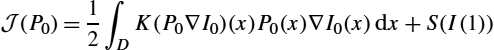
Hereafter we discuss the work presented in [19,7]. In most applications a Gaussian kernel is used to smooth the deformations. A kernel corresponding to the differential operator (Id+ηΔ)k![]() for a well-chosen k with a single parameter η may also be used. The Gaussian width σ is commonly chosen to obtain a good matching accuracy. This means that small values, close to the image resolution, are used for σ. We can then wonder what is the effect of this parameter on the structure of the deformation. In [19] we have illustrated the influence of σ on the mapping obtained between two images of the grey matter acquired on a preterm baby at about 36 and 43 weeks of gestational age, as summarized in Fig. 14.2. Let us focus on the (B-top) subfigure of Fig. 14.2. The yellow (ligth gray in print version) isoline represents the cortex boundary in a 2D region of interest (ROI) out of a 3D segmented image S36
for a well-chosen k with a single parameter η may also be used. The Gaussian width σ is commonly chosen to obtain a good matching accuracy. This means that small values, close to the image resolution, are used for σ. We can then wonder what is the effect of this parameter on the structure of the deformation. In [19] we have illustrated the influence of σ on the mapping obtained between two images of the grey matter acquired on a preterm baby at about 36 and 43 weeks of gestational age, as summarized in Fig. 14.2. Let us focus on the (B-top) subfigure of Fig. 14.2. The yellow (ligth gray in print version) isoline represents the cortex boundary in a 2D region of interest (ROI) out of a 3D segmented image S36![]() , and the ROI is located in the red square of the (A-bottom) subfigure. The grey levels of the same (B-top) subfigure also represent the segmented cortex in the same preterm baby but 7 weeks later. It is obvious that the brain became globally larger as the brain and the skull strongly grow at this age. The shapes should be almost translated at the scale of this ROI to capture the amplitude of the deformation. It is important that existing cortex folds also became deeper and new folds appeared, which is normal during brain maturation because the cortex growth is faster than the skull growth. Capturing the folding process requires registering the images at a scale close to the image resolution here. To conclude, the registration of these images requires at a same time a large σ and a small σ. If only a small σ is used, then optimal path (and the optimization process) will lead to physiologically implausible deformations. This is obvious in Fig. 14.2(C), where the brown isoline represents the boundaries of the deformed voxels after registration. In this example the volume of some voxels becomes huge, and other voxels almost disappear. If this deformation was the real one, then the studied brain would have a strongly heterogeneous development in space, which is clearly not realistic. On the contrary, if only a large σ was used, then the optimal path would not capture fine deformations, as shown in Fig. 14.2(D). This justifies the use of multiscale kernels to establish geodesics between such follow-up medical images.
, and the ROI is located in the red square of the (A-bottom) subfigure. The grey levels of the same (B-top) subfigure also represent the segmented cortex in the same preterm baby but 7 weeks later. It is obvious that the brain became globally larger as the brain and the skull strongly grow at this age. The shapes should be almost translated at the scale of this ROI to capture the amplitude of the deformation. It is important that existing cortex folds also became deeper and new folds appeared, which is normal during brain maturation because the cortex growth is faster than the skull growth. Capturing the folding process requires registering the images at a scale close to the image resolution here. To conclude, the registration of these images requires at a same time a large σ and a small σ. If only a small σ is used, then optimal path (and the optimization process) will lead to physiologically implausible deformations. This is obvious in Fig. 14.2(C), where the brown isoline represents the boundaries of the deformed voxels after registration. In this example the volume of some voxels becomes huge, and other voxels almost disappear. If this deformation was the real one, then the studied brain would have a strongly heterogeneous development in space, which is clearly not realistic. On the contrary, if only a large σ was used, then the optimal path would not capture fine deformations, as shown in Fig. 14.2(D). This justifies the use of multiscale kernels to establish geodesics between such follow-up medical images.
14.2.2 Multiscale kernels
As for the LDDMM model, we recall that the kernel spatially interpolates the rest of the information (i.e., the momentum) to drive the motion of the points where there is no gradient information, for example, in flat image regions. Therefore it is natural to introduce a sum of kernels to fill in the missing information while preserving the physiologically realistic matchings. Therefore more plausible deformations are obtained since the correlation of the motions of the points is higher.
In practice this method works really well, and the mathematical insight for its efficiency is probably the variational interpretation of the sum of kernel, explained hereafter. For simplicity, we only treat the case of a finite set of RKHS Hilbert spaces Hi![]() with kernels ki
with kernels ki![]() and Riesz isomorphisms Ki
and Riesz isomorphisms Ki![]() between H⁎i
between H⁎i![]() and Hi
and Hi![]() for i=1,…,n
for i=1,…,n![]() . For every i, Hi
. For every i, Hi![]() is a subspace of the space of C1
is a subspace of the space of C1![]() vector fields on the domain D. Denoting H=H1+…+Hn
vector fields on the domain D. Denoting H=H1+…+Hn![]() , the space of all functions of the form v1+…+vn
, the space of all functions of the form v1+…+vn![]() with vi∈Hi
with vi∈Hi![]() , the norm is defined by
, the norm is defined by
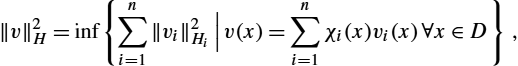
‖v‖2H=inf{n∑i=1‖vi‖2Hi|n∑i=1vi=v}.

The minimum is achieved for a unique n-tuple of vector fields, and the space H endowed with the norm defined by (14.15) is complete. The result is the following: there exists a unique element p∈⋂ni=1H⁎i![]() for which we have vi=Kip
for which we have vi=Kip![]() and
and
v=n∑i=1Kip,

the family (vi)i=1,…,n![]() realizing the (unique) infimum of the variational problem (14.15). Formula (14.15) induces a scalar product on H, which makes H an RKHS, and its associated kernel is k:=∑ni=1ki
realizing the (unique) infimum of the variational problem (14.15). Formula (14.15) induces a scalar product on H, which makes H an RKHS, and its associated kernel is k:=∑ni=1ki![]() , where ki
, where ki![]() denotes the kernel of the space Hi
denotes the kernel of the space Hi![]() . This property was written in [3] and is standard in convex analysis. Indeed, note that this property is the particular case of an elementary result in convex analysis, at least in finite dimensions: the convex conjugate of an infimal convolution is equal to the sum of the convex conjugates [20].
. This property was written in [3] and is standard in convex analysis. Indeed, note that this property is the particular case of an elementary result in convex analysis, at least in finite dimensions: the convex conjugate of an infimal convolution is equal to the sum of the convex conjugates [20].
Another phenomenon observed in practice is that a better quality of matching is obtained with a sum of kernels than with a single kernel of small width. Although we have no quantitative argument in this direction, we strongly believe that this is due to the convergence of the gradient descent algorithm to local minima. In standard image registration, coarse to fine techniques [11] are ubiquitous. They consist in first registering two images with a strong regularization level and then iteratively decreasing the regularization level when the algorithm has converged at the current scale. At each considered scale, gradient descent-based registration is then likely to be performed in a stable orbit with respect to the compared shape scale. In LDDMM, using the sum of kernels at different scales instead of small scales only may then have a similar effect from an optimization point of view.
Based on the practical implementation of LDDMM for images of [6] and summarized Algorithm 14.1, we have proposed to use smoothing kernels constructed as the sum of several Gaussian kernels [19]. These kernels, denoted by MK, that are the weighted sums of N Gaussian kernels Kσn![]() , each of them being parameterized by its standard deviation σn
, each of them being parameterized by its standard deviation σn![]() :
:
MK(x)=N∑n=1anKσn(x)=N∑n=1an(2π)−3/2|Σn|−1/2exp(−12xTΣ−1nx),
where Σn![]() and an
and an![]() are respectively the covariance matrix and the weight of the nth Gaussian function. Each Σn
are respectively the covariance matrix and the weight of the nth Gaussian function. Each Σn![]() is only defined by a characteristic scale σn
is only defined by a characteristic scale σn![]() : Σn=σnIdRd
: Σn=σnIdRd![]() . Once this kernel is defined, the registration algorithm is the same as in Algorithm 14.1.
. Once this kernel is defined, the registration algorithm is the same as in Algorithm 14.1.
A tricky aspect of this kernel construction for practical applications is however the tuning of their weights an![]() . Although the choice of the σn
. Although the choice of the σn![]() has a rather intuitive influence on the optimal deformations, the tuning of the an
has a rather intuitive influence on the optimal deformations, the tuning of the an![]() strongly depends on the representation and the spatial organization of the registered shapes at the scales σn
strongly depends on the representation and the spatial organization of the registered shapes at the scales σn![]() , n∈[1,N]
, n∈[1,N]![]() . As described in [19], it depends on: (1) Representation and spatial organization of the structures: A same shape can be encoded in various ways. For instance, it can be a binary or a grey-level image. This representation has first a nonlinear influence on the similarity metric (the sum of squared differences in LDDMM) forces (unsmoothed gradients) as shown line 12 of Algorithm 14.1. The choice of optimal parameters an
. As described in [19], it depends on: (1) Representation and spatial organization of the structures: A same shape can be encoded in various ways. For instance, it can be a binary or a grey-level image. This representation has first a nonlinear influence on the similarity metric (the sum of squared differences in LDDMM) forces (unsmoothed gradients) as shown line 12 of Algorithm 14.1. The choice of optimal parameters an![]() is even more complicated to do as the spatial relation between the shape structures should also be taken into account when smoothing the forces (line 13 of Algorithm 14.1). (2) Prior knowledge: Prior knowledge about the amplitude of the structures displacement at each scale σn
is even more complicated to do as the spatial relation between the shape structures should also be taken into account when smoothing the forces (line 13 of Algorithm 14.1). (2) Prior knowledge: Prior knowledge about the amplitude of the structures displacement at each scale σn![]() may be incorporated in an
may be incorporated in an![]() .
.
In [17] we have proposed to semiautomatically tune the an![]() as follows:
as follows:
an=a′n/g(Kσn,IS,IT),
where g(Kσn,IS,IT)![]() represents the typical amplitude of the forces when registering IS
represents the typical amplitude of the forces when registering IS![]() to IT
to IT![]() at a scale σn
at a scale σn![]() . This amplitude is related to (1) and cannot therefore be computed analytically. An empirical technique to tune it is the following: for each Kσn
. This amplitude is related to (1) and cannot therefore be computed analytically. An empirical technique to tune it is the following: for each Kσn![]() , the value of g(Kσn,IS,IT)
, the value of g(Kσn,IS,IT)![]() can be estimated by observing the maximum update of the velocity field v in a preiteration of registration of IS
can be estimated by observing the maximum update of the velocity field v in a preiteration of registration of IS![]() on IT
on IT![]() using only the kernel Kσn
using only the kernel Kσn![]() with an=1
with an=1![]() . The apparent weights a′n
. The apparent weights a′n![]() , n∈[1,N]
, n∈[1,N]![]() , provide an intuitive control of the amplitude of the displacements and are related to (2). To deform the largest features of IS
, provide an intuitive control of the amplitude of the displacements and are related to (2). To deform the largest features of IS![]() and IT
and IT![]() with a similar amplitude at each scale σn
with a similar amplitude at each scale σn![]() , the user should tune all the apparent weights a′n
, the user should tune all the apparent weights a′n![]() with the same value. Typical results we obtained in [19] on the example of Fig. 14.2 are shown in Fig. 14.3. They make clear the fact that multiscale kernels with automatically tuned an
with the same value. Typical results we obtained in [19] on the example of Fig. 14.2 are shown in Fig. 14.3. They make clear the fact that multiscale kernels with automatically tuned an![]() following our method efficiently solved the problem we initially described.
following our method efficiently solved the problem we initially described.

 having the same value.
14.2.3 Distinguishing the deformations at different scales
It is interesting to remark that the influence of each subkernel of the multiscale kernels we defined can be measured. Distinguishing scale-dependent deformations is indeed useful for further statistical analysis. A first attempt to characterize this influence has been presented in [19] and was strongly developed in [7]. The main contribution of [7] was to formulate the multiscale LDDMM registration with a semidirect product. Registering IS![]() on IT
on IT![]() is then done by minimizing a registration energy EN
is then done by minimizing a registration energy EN![]() with respect to the N-tuple (v1,…,vN)
with respect to the N-tuple (v1,…,vN)![]() where each time-dependent velocity field vn
where each time-dependent velocity field vn![]() is associated with scale-dependent deformations. Then the minimized energy is
is associated with scale-dependent deformations. Then the minimized energy is
EN(v1,…,vN)=12N∑n=1∫10‖vn(t)‖2Hndt+S(IS,IT,φ),

where the space Hn![]() corresponds to the kernel Kσn
corresponds to the kernel Kσn![]() , and φn(t)
, and φn(t)![]() is defined by
is defined by
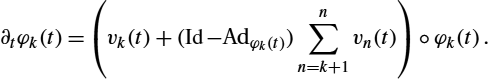
∂tφk(t)=(vk(t)+(Id−Adφk(t))n∑n=k+1vn(t))∘φk(t).
Here Adφv![]() also denotes the adjoint action of the group of diffeomorphisms on the Lie algebra of vector fields:
also denotes the adjoint action of the group of diffeomorphisms on the Lie algebra of vector fields:
Adφv(x)=(Dφ.v)∘φ−1(x)=Dφ−1(x)φ.v(φ−1(x)).
These equations then allow us to quantify scale-dependent deformations φn![]() in the whole deformation φ. We can also sum over all scales to form v(t)=∑nk=1vk(t)
in the whole deformation φ. We can also sum over all scales to form v(t)=∑nk=1vk(t)![]() and compute the flow φ(t)
and compute the flow φ(t)![]() of v(t)
of v(t)![]() . A simple calculation finally shows that
. A simple calculation finally shows that
φ(t)=φ1(t)∘…∘φn(t).
Results and algorithmic description of the solution for 3D images were given [7]. An illustration of this paper, where the deformations between two brain images were split into 7 scales, is given Fig. 14.4. Note also that in [21] the authors build on these ideas of multiscale kernels and incorporate some sparsity prior. On the other hand, we can extend the space of kernels as done in [24], in which the authors construct multiscale kernels based on wavelet frames and with an apparent improvement of the registration results, although the corresponding group structure interpretation is possibly lost.

14.3 Sliding motion constraints
14.3.1 Introduction
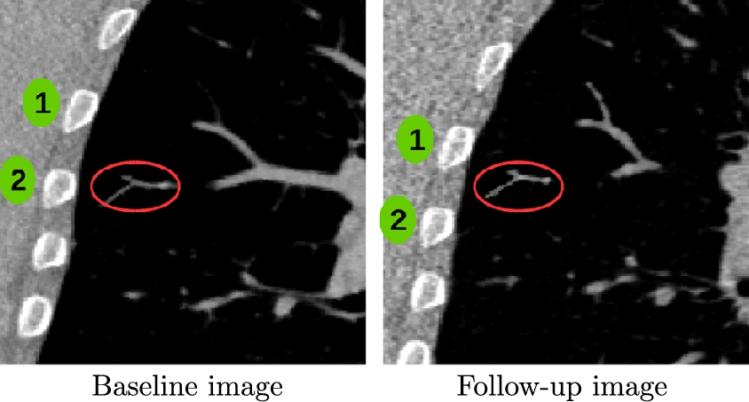
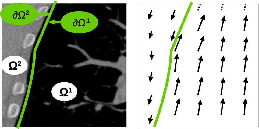
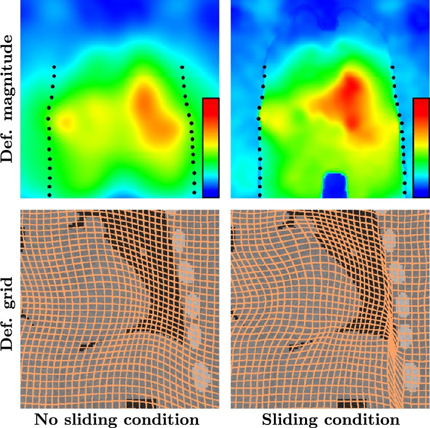
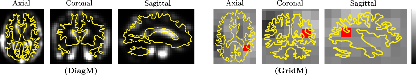
Now we focus on how to model sliding constraints in the LDDMM formalism. Such constraints are observed, for example, at the lung boundaries, as emphasized in Fig. 14.5. In [18] we have developed a smoothing strategy to solve this problem by using Algorithm 14.1 (of [6]) with specific smoothing properties. The central idea is to predefine different regions of interest Ωk![]() in the domain Ω of the registered images at the boundary of which discontinuous deformations will be potentially estimated. Note first that these regions of interest are fixed so the source image IS
in the domain Ω of the registered images at the boundary of which discontinuous deformations will be potentially estimated. Note first that these regions of interest are fixed so the source image IS![]() and the target image IT
and the target image IT![]() should be aligned at the boundaries of the regions Ωk
should be aligned at the boundaries of the regions Ωk![]() , which is done in Algorithm 14.1 by using a standard registration strategy with large amount of smoothing. This domain decomposition is illustrated Fig. 14.6.
, which is done in Algorithm 14.1 by using a standard registration strategy with large amount of smoothing. This domain decomposition is illustrated Fig. 14.6.
14.3.2 Methodology
Instead of considering a reproducing kernel Hilbert apace (RKHS) V embedded in C1(Ω,Rn)![]() or W1,∞
or W1,∞![]() as in the previous section, here we use N RKHS of vector fields Vk∈C1(Ωk,[0,1])
as in the previous section, here we use N RKHS of vector fields Vk∈C1(Ωk,[0,1])![]() , which can capture sliding motion, that is, with an orthogonal component to the boundary that vanishes at any point of ∂Ωk
, which can capture sliding motion, that is, with an orthogonal component to the boundary that vanishes at any point of ∂Ωk![]() . The set of admissible vector fields is therefore defined by V:=⨁Nk=1Vk
. The set of admissible vector fields is therefore defined by V:=⨁Nk=1Vk![]() , the direct sum of the Hilbert spaces (Vk)k∈〚1,N〛
, the direct sum of the Hilbert spaces (Vk)k∈〚1,N〛![]() . In particular, the norm on V of a vector field vt
. In particular, the norm on V of a vector field vt![]() is given by
is given by
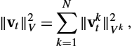
‖vt‖2V=N∑k=1‖vkt‖2Vk,
where vkt![]() is the restriction of vt
is the restriction of vt![]() to Ωk
to Ωk![]() . The flow of any v∈L2([0,1],V)
. The flow of any v∈L2([0,1],V)![]() is then well defined although the resulting deformations are piecewise diffeomorphic and not diffeomorphic. As a consequence, the deformation is a diffeomorphism on each subdomain and allows for sliding motion along the boundaries.
is then well defined although the resulting deformations are piecewise diffeomorphic and not diffeomorphic. As a consequence, the deformation is a diffeomorphism on each subdomain and allows for sliding motion along the boundaries.
Now that an admissible RKHS is defined, let us focus on the strategy we used to mimic the Gaussian smoothing of the updates u (see line 13 in Algorithm 14.1) with the desired properties. We use the heat equation to smooth u in each region Ωk![]() : ∂u/∂τ=Δu
: ∂u/∂τ=Δu![]() , where τ∈[0,Γ]
, where τ∈[0,Γ]![]() is a virtual diffusion time. We denote by ∂Ωk
is a virtual diffusion time. We denote by ∂Ωk![]() the boundaries of Ωk
the boundaries of Ωk![]() . Here Γ controls the amount of smoothing. To prevent from information exchange between the different regions, Neumann boundary conditions are additionally modeled at each point x of ∂Ωk
. Here Γ controls the amount of smoothing. To prevent from information exchange between the different regions, Neumann boundary conditions are additionally modeled at each point x of ∂Ωk![]() : ∇u(x)⋅n(x)=0
: ∇u(x)⋅n(x)=0![]() , where n(x)
, where n(x)![]() is normal to ∂Ωk
is normal to ∂Ωk![]() at x. Independent Gaussian based convolution in each region Ωk
at x. Independent Gaussian based convolution in each region Ωk![]() , would have been a quicker alternative in terms of computations but would not take into account the intrinsic region geometry. Then, to ensure that the orthogonal component to the boundary vanishes at any point of ∂Ωk
, would have been a quicker alternative in terms of computations but would not take into account the intrinsic region geometry. Then, to ensure that the orthogonal component to the boundary vanishes at any point of ∂Ωk![]() , we use a projection strategy of the updates before and after smoothing so that they respect this constraint.
, we use a projection strategy of the updates before and after smoothing so that they respect this constraint.
To do so, we consider the vector field T so that for each point x∈Ω![]() , x+T(x)
, x+T(x)![]() is the nearest boundary between two subdomains in a limited neighborhood around the boundaries ∂Ωk
is the nearest boundary between two subdomains in a limited neighborhood around the boundaries ∂Ωk![]() . For the registration of pulmonary images, we empirically use a neighborhood of about γ=20
. For the registration of pulmonary images, we empirically use a neighborhood of about γ=20![]() millimeters. Consider a velocity field w defined on Ω. We use T to enforce the sliding conditions around ∂Ωk
millimeters. Consider a velocity field w defined on Ω. We use T to enforce the sliding conditions around ∂Ωk![]() by reducing the contributions of w(x)
by reducing the contributions of w(x)![]() in the direction of T(x)
in the direction of T(x)![]() when ||T(x)||L2<γ
when ||T(x)||L2<γ![]() :
:
w(x)=w(x)−α(x)T(x)<w(x),T(x)>L2||T(x)||2L2,

where the weight α(x)![]() equals (γ−||T(x)||)2/γ
equals (γ−||T(x)||)2/γ![]() . For numerical stability, w(x)
. For numerical stability, w(x)![]() is set to 0 if ||T(x)||2L2=0
is set to 0 if ||T(x)||2L2=0![]() . The registration algorithm is then the same as Algorithm 14.1 except line 13, where u is first projected using Eq. (14.23), then smoothed using the heat (diffusion) equation, and then projected again using Eq. (14.23).
. The registration algorithm is then the same as Algorithm 14.1 except line 13, where u is first projected using Eq. (14.23), then smoothed using the heat (diffusion) equation, and then projected again using Eq. (14.23).
14.3.3 Results and discussion
Results shown in [18] make clear the impact of this strategy compared with standard smoothing kernels. Fig. 14.7 shows the impact of such a piecewise diffeomorphic kernel when registering lung image where a sliding motion is clearly required at the lung boundaries. Note that to make this strategy tractable on large medical images (as in Fig. 14.7), we also coded it in the LogDemons formalism of [26]. This formalism is indeed less memory consuming than LDDMM, as the diffeomorphisms are encoded in stationary velocity fields and not time-dependent ones as in LDDMM. Computational burden would be too high in the LDDMM framework. However, both LogDemons and LDDMM with the proposed sliding motion estimation strategy led to similar results on smaller images.
14.4 Left-invariant metrics
14.4.1 Introduction
In this section, we describe the results obtained in [22,23]. A natural extension of the sum of kernels consists in having a kernel that may depend on the location. However, the right-invariant point of view is meant for a homogeneous material whose properties are translation invariant although this is not required by the theory. In practice the kernel used in diffeomorphic methods has always been chosen to be translationally invariant and isotropic. In LDDMM spatially adaptive or nonisotropic (“direction-dependent”) kernels have no obvious interpretation, because the norm is defined in Eulerian coordinates, so that as t varies during the deformation, a fixed point in the source image moves through space, and conversely, a fixed point in space will correspond to different points in the source image. Similarly, the directions in a direction-dependent kernel are defined with respect to Eulerian coordinates, not the coordinates of the moving source image. Nonetheless, spatially adaptive kernels are potentially of great interest in medical applications if they can be made to represent spatially variable (or nonisotropic) deformability of tissue. This is indeed already done in [16] to model sliding conditions between the lungs and the ribs. In this section we present a slightly different registration framework than LDDMM, which naturally supports the use of spatially adaptive kernels.
14.4.2 Methodology
The proposed framework is based on a left-invariant metric on the group of deformations, where its name LIDM (left-invariant diffeomorphic metrics) comes from. Left-invariance means that this metric satisfies, in a smooth setting, the following property: For all elements ψ1![]() , ψ2
, ψ2![]() , ψ3
, ψ3![]() in the group,
in the group,
dist(ψ3∘ψ1,ψ3∘ψ0)=dist(ψ1,ψ0),
which is in contrast with formula (14.7). In fact, such a left-invariant metric is based on a choice of norm in the body (Lagrangian) coordinates of the source image. This means that instead of the V norm applied to the spatial velocity defined by (14.12), it is applied to the convective velocity v(t)![]() implicitly defined by
implicitly defined by
∂tφ(t)=dφ(t)⋅v(t),
where dφ(t)![]() is the spatial derivative of φ(t)
is the spatial derivative of φ(t)![]() .
.
It is well known that left- and right-invariant metrics are isometric by the inverse map. Therefore, as expected, we obtain the following result.
Corollary 14.1
[Equivalence between LIDM and LDDMM] Consider the problem of minimizing
JIT(φ)=12∫10‖v(t)‖2Vdt+E(IS∘φ−11,IT)
for φ0=IdΩ![]() , and with constraint either
, and with constraint either
∂tφt=dφt⋅vt(LIDM constraint)
or
∂tφt=vt∘φt(LDDMM constraint).
Then
- 1. The optimal endpoint
 is the same with either constraint.
 - 2. If
 minimizes
  in LIDM, then
  minimizes in LDDMM.
 - 3. If
 minimizes in LDDMM, then
  minimizes in LIDM.
Although not surprising, this result gives a mathematical interpretation to the use of spatially adaptive kernels that can be defined using a variational approach. Let us consider, as in the previous section, a family of RKHS ![]() and an operator
and an operator ![]() . On the space H we introduce
. On the space H we introduce
Using again duality and under mild assumptions, the kernel associated with H is ![]() .
.
Let us give an instance of it in the context of biomedical images. Suppose we have a partition of unity (![]() ) of the domain of interest (a manual segmentation of the biological shape) where we have some knowledge of the deformability properties of the shape modeled by the kernel
) of the domain of interest (a manual segmentation of the biological shape) where we have some knowledge of the deformability properties of the shape modeled by the kernel ![]() . The map A can be chosen as
. The map A can be chosen as ![]() , and the corresponding kernel is
, and the corresponding kernel is
This kernel satisfies the embedding condition under mild conditions on the element of the partition of unity ![]() .
.
14.4.3 Results and discussion
The experiment of Fig. 14.8 is adapted from [22], and it shows registration results for a synthetic example, which includes features at different scales. LIDM shows the results of the registration using a kernel defined accordingly to the partition of unity shown in the figure (two Gaussian kernels with a large σ on the white and a small σ on the black). As expected, it performs better than the sum of kernel because it captures the small scale deformations.

The use of spatially adaptive kernels provably improves the registration results on real data. However, the shortcoming of this approach is that the kernel does not evolve with the deformed shape. For small/medium deformations, it may not be a problem, but it cannot be applied in the case of large deformations. In such a case the kernel has to depend on the shape itself. Such approaches have actually been developed in [30,4,2], where the operator A depends on the shape itself, but developing models for images associated with an efficient implementation remains open.
14.5 Open directions
14.5.1 Learning the metric
There are two different point of views that can be developed to improve on the results of LDDMM: On the one hand, incorporating mechanical or biological constraints to reproduce more realistic results is what we have described so far in this chapter. On the other hand, it is also natural to learn the metric parameters using data driven methods if no mechanical model is well established for the data of interest. Instead of having a partition of unity drawn by the user, it is also natural to ask whether the smoothing kernel can be learned from data. We summarize here an approach proposed in [27] to learn the parameters from a given population and a given template.
Building on the LIDM model, we aim at designing a set of kernels expressing spatially adaptive metrics. We use (symmetric) positive definite matrices M as a parameterization of this set of kernels. To ensure the smoothness of the deformations, any kernel of this set has to satisfy the constraint that the Hilbert space of vector fields is embedded in the Banach space of ![]() vector fields. To enforce this constraint, we propose the following parameterization:
vector fields. To enforce this constraint, we propose the following parameterization:
where ![]() is a spatially homogeneous smoothing kernel (typically Gaussian). Now the variational model consists in minimizing the functional with a positive real β:
is a spatially homogeneous smoothing kernel (typically Gaussian). Now the variational model consists in minimizing the functional with a positive real β:
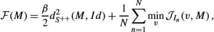
where M is symmetric. The first term is a regularizer of the kernel parameters so that the minimization problem is well posed. Here, it favors parameterizations of M close to the identity matrix, but other a priori correlation matrix could be used. The term ![]() can be chosen as the squared distance on the space of positive definite matrices given by
can be chosen as the squared distance on the space of positive definite matrices given by ![]() . Here again other choices of regularizations could have been used such as the log-determinant divergence. This model has been implemented in [27], where a simple method of dimension reduction was used since the matrix M is of size
. Here again other choices of regularizations could have been used such as the log-determinant divergence. This model has been implemented in [27], where a simple method of dimension reduction was used since the matrix M is of size ![]() , where n is the number of voxels, and it gave promising results on the 40 subjects of the LONI Probabilistic Brain Atlas (LPBA40). An illustration of the matrix M we computed in this paper is given in Fig. 14.9.
, where n is the number of voxels, and it gave promising results on the 40 subjects of the LONI Probabilistic Brain Atlas (LPBA40). An illustration of the matrix M we computed in this paper is given in Fig. 14.9.
Another possible direction as done in [14] consists in learning the partition of unity ![]() with some smoothness constraints on the
with some smoothness constraints on the ![]() such as
such as ![]() or TV. Moreover, since there is an interplay in the optimality equations between the gradient of the deformed image and the deformation, it is possible to introduce some information on the regularization of the partition so that it takes into account this interplay.
or TV. Moreover, since there is an interplay in the optimality equations between the gradient of the deformed image and the deformation, it is possible to introduce some information on the regularization of the partition so that it takes into account this interplay.
14.5.2 Other models
From a methodological point of view, the main weakness of the previously presented methods is probably the fact that the metric does not evolve with the shape in Lagrangian coordinates. To make the practical impact of this property clear, assume that a part of the shape follows a fixed volume transformation. In that case the models proposed are clearly unadapted as they cannot incorporate this property. This is why constrained diffeomorphic evolutions have been introduced in the literature [30,2]. Most of the time these constraints are incorporated in Lagrangian coordinates such as in [10]. However, fast computational methods for diffeomorphic image matching are designed in Eulerian coordinates; see, for instance, [31,12]. We propose an Eulerian-based PDE model, which can be seen as a mild modification of the LDDMM framework presented, incorporating the modeling assumption that the metric is naturally image dependent.
The standard formulation of shape-dependent metric registration is similar to the formulation in (14.1) when the norm on the vector field v depends on the current shape I. It is important that it is often possible to preserve the metric property in this type of modification. The manifold Q that we are going to consider consists in augmenting the template image I with a partition of unity ![]() . The definition of the action of φ in the group of diffeomorphisms is as follows:
. The definition of the action of φ in the group of diffeomorphisms is as follows:
In other words, we consider the partition of unity as additional images that are advected by the flow. The variational problem is then the following:

where the norm is as in Eq. (14.29), that is,
and the flow is defined by

Alternatively, functional (14.34) can be rewritten using a shape-dependent metric using the Lagrange multiplier method, and it is similar to the constrained evolutions proposed in [30]. The optimality equation can be written as

Note that the Lagrange multiplier associated with the partition evolves accordingly to the fourth equation in (14.37), which has a source term on its right-hand side that differs from the optimality equations (14.12).