
A discretize–optimize approach for LDDMM registration
Thomas Polzina; Marc Niethammerb,c; François-Xavier Vialardd; Jan Modersitzkia,e aInstitute of Mathematics and Image Computing, University of Lübeck, Lübeck, Germany
bDepartment of Computer Science, University of North Carolina at Chapel Hill, Chapel Hill, NC, United States
cBiomedical Research Imaging Center (BRIC), Chapel Hill, NC, United States
dLaboratoire d'informatique Gaspard Monge, Université Paris-Est Marne-la-Vallée, UMR CNRS 8049, Champs sur Marne, France
eFraunhofer MEVIS, Lübeck, Germany
Abstract
Large deformation diffeomorphic metric mapping (LDDMM) is a popular approach for deformable image registration with nice mathematical properties. LDDMM encodes spatial deformations through time-varying velocity fields. Hence registration requires optimization over these time-varying velocity fields, resulting in a large-scale constrained optimization problem.
Typical numerical solution approaches for LDDMM use an optimize–discretize strategy, where optimality conditions are derived in the continuum and subsequently discretized and solved. Here we explore solution methods based on the discretize–optimize approach and discuss ramifications for popular LDDMM relaxation and shooting approaches. The focus is on a consistent method that uses the appropriate Runge–Kutta methods for the solution of all arising PDEs in the Eulerian frame. Additionally, we discuss both run-time and memory consumption requirements and present an approach that makes the registration suitable for standard PCs. We demonstrate the practicality of our proposed approach in the context of image registration applied to 3D computed tomography (CT) scans of the lung.
Keywords
LDDMM; Discretize–Optimize; Image Registration; Optimal Control; Lung; Computed Tomography; Runge–Kutta Methods
13.1 Introduction
The goal of image registration is to establish spatial correspondences between images. Image registration is a challenging but important task in image analysis. In particular, in medical image analysis image registration is a key tool to compare patient data in a common space, to allow comparisons between pre-, inter-, or post-intervention images, or to fuse data acquired from different and complementary imaging devices such as positron emission tomography (PET), computed tomography (CT), or magnetic resonance imaging (MRI) [56].
Image registration is of course not limited to medical imaging, but is important for a wide range of applications; for example, it is used in astronomy, biology/genetics, cartography, computer vision, and surveillance. Consequently, there exists a vast number of approaches and techniques; see, for example, [10,29,31,33,44,56,65,66,84,87,91,97,109] and references therein.
Optical flow approaches [48,55] are popular and commonly used in computer vision [12,100,72,106,11]. However, computer vision applications typically have different requirements regarding spatial transformations than medical image analysis applications. For example, when processing natural images, objects, such as cars or people, should typically be allowed to move independently of the background. However, in many medical applications it is natural to constrain the sought-for mapping to be bijective or even diffeomorphic. In early days of image registration, transformation models were (and sometimes still are) constricted to rigid mappings, which obviously fulfill this constraint. However, more flexible, for example, deformable, transformation models are required to capture subtle localized changes. Early work on deformable image registration includes variational approaches based on elasticity theory [30,9,6], where a spatial transformation is represented nonparametrically (via a deformation field) and is regularized through an elastic potential function.
The mathematical reason for introducing the regularizer is to ensure solutions of the variational formulation. It may also be interpreted as a penalty for nonelasticity. Elastic registration has been widely and successfully used. However, an elastic regularizer can in general not guarantee that a computed mapping is bijective [23]. To ensure bijectivity, one may add constraints to a registration formulation. Alternatively, one can formulate a registration model that by construction guarantees the regularity of the transformation. Examples for the former approach are [79,36,37]. While Rohlfing et al. [79] employed an additional penalty term on the determinant of the Jacobian of the transformation that improves transformation regularity but cannot guarantee bijective mappings, Haber and Modersitzki developed similar ideas, but with equality [36] or box constraints [37] thereby guaranteeing bijectivity. Nevertheless, Haber and Modersitzki still use a mathematical model based on linear elasticity theory, which is only appropriate for small deformations. As convex energies, such as the linear elastic potential, result in finite penalties, they are insufficient to guarantee one-to-one maps [13,24]. Therefore Burger et al. [13] used hyperelasticity and quasiconvex functions to obtain a registration model yielding bijective transformations while allowing for large deformations.
Another possibility to ensure diffeomorphic mappings (smooth mappings that are bijective and have a smooth inverse) is to express a transformation implicitly through velocity fields. The intuitive idea is that it is easy to ensure diffeomorphic transformations for small-scale displacements by using a sufficiently strong spatial regularization. Hence a complex diffeomorphic transform can be obtained, capturing large displacements, as the composition of a large or potentially infinite number of small-scale diffeomorphisms. These small-scale diffeomorphisms in turn can be obtained by integrating a static or time-dependent velocity field in time. Early work explored such ideas in the context of fluid-based image registration [23]. In fact, for approaches using velocity fields, the same regularizers as for the small displacement registration approaches (based on elasticity theory or the direct regularization of displacement fields) can be used. However, the regularizer is now applied to one or multiple velocity fields instead of a displacement field, and the transformation is obtained via time-integration of the velocity field.
The solution of the arising problems is computationally expensive, as in the most general case we now need to estimate a spatio-temporal velocity field instead of a static displacement field. Greedy solution approaches as well as solutions based on a stationary velocity field have been proposed to alleviate the computational burden (both in computational cost, but also with respect to memory requirements) [23,1,2,57]. However, these methods in general do not provide all the nice mathematical properties (metric, geodesics, etc.) of the nongreedy large deformation diffeomorphic metric mapping (LDDMM) registration approach [61], which we will explore numerically here.
Various numerical approaches have been proposed for LDDMM, for example, [23,61,96,7]. Traditionally, relaxation formulations [7] have been used to solve the LDDMM optimization problem. Here, one directly optimizes over spatio-temporal velocity fields, ensuring that the velocity field at any given time is sufficiently smooth. The resulting transformation, obtained via time-integration of the spatio-temporal velocity field, is used to deform the source image such that it becomes similar to the target image. Specifically, the LDDMM relaxation formulation is solved via an optimize–discretize approach [7], where a solution to the continuous time optimality conditions for the associated constrained optimization problem (the constraint being the relation between the spatial transformation and the velocity fields) is computed. These optimality conditions are the Euler–Lagrange equations corresponding to the constrained optimization problem and can be regarded as the continuous equivalent of the Karush–Kuhn–Tucker (KKT) [71, p. 321] equations of constrained optimization. To numerically determine a solution fulfilling the Euler–Lagrange equations, one uses an adjoint solution approach, which allows the efficient computation of the gradient of the LDDMM relaxation energy with respect to the spatio-temporal velocity field via a forward/backward sweep. This gradient can then be used within a gradient descent scheme or as the basis of sophisticated numerical solution approaches. Note that the adjoint solution approach is, for example, also at the core of the famous backpropagation algorithm for the training of neural networks [54] or the reverse mode of automatic differentiation [34, pp. 37].1 For an LDDMM relaxation solution, a geodesic path (fulfilling the Euler–Lagrange equations exactly) is only obtained at convergence [7].
More recently, shooting approaches like [3,98,70] have been proposed. Again, an optimize–discretize approach is used. Here, instead of numerically solving the Euler–Lagrange equations of the LDDMM energy (which can alternatively be represented via the Euler–Poincaré diffeomorphism equation [62] (EPDiff)), these Euler–Lagrange equations are imposed as a dynamical system, and the LDDMM energy is reformulated as an initial value problem. Hence all paths obtained during the optimization process are by construction geodesics—they may just not be the optimal ones. The price to pay for such a reduced parameterization is that one now optimizes over a second-order partial differential equation that describes the geodesic path. A simple analogy in the one-dimensional Euclidean space is that in relaxation, registration between two points is performed over all possible paths leading at convergence to a straight-line path. On the contrary, for shooting, we already know that the optimal solution should be a straight line, and consequentially optimization is only performed regarding the line slope and y-intercept.
Although the mathematical framework for LDDMM is very appealing, its numerical treatment is not trivial, may lead to nondiffeomorphic transformations, and is highly demanding both in terms of memory and computational costs. As discussed before, current LDDMM solutions are mainly based on optimize–discretize formulations, that is, optimality conditions are derived in continuous space and then discretized [7,62]. Not surprisingly, it is possible that a solution of the discrete equations is an optimizer neither for discrete nor for continuous energy [35].
Hence the goal of this chapter is to develop a discretize–optimize approach for LDDMM, where the starting point is the discretization of the energy functional. Consequentially, solutions to the associated optimality conditions are indeed optimizers of the discretized energy. Additionally, we integrate a suitable interpolation operator [51] into the LDDMM framework to reduce computational demands and memory consumption without losing registration accuracy. Furthermore, we use the so-called normalized gradient fields (NGF) distance measure, which is designed to align image edges [38,66]. NGF has been successfully applied to lung CT registration [81,51,74–76,82], which is one of our example applications in Section 13.8.
The chapter is organized as follows. In Section 13.2 the LDDMM concept is introduced, and two approaches [7,45] used for solving the constrained optimization problems are discussed. In Section 13.3 we extend these models, discuss the shooting approach, and formulate them in the context of general distance measures for images. For simplicity, Section 13.4 discusses the discretization of the models in the one-dimensional case. This allows introducing the basic ingredients (grids, regularization, derivatives, transport equation, etc.) required for the 3D formulation in a compact manner. In Section 13.5 we address the discretization and solution of the partial differential equations constraining the LDDMM models (e.g., the transport equations) via Runge–Kutta methods. The extension of the described formalism to 3D is given in Section 13.6. In Section 13.7 details on the numerical optimization and the solution of the optimization problems in a multilevel approach are provided. Afterward, in Section 13.8 we evaluate the performance of the proposed methods and present experimental results. Finally, we conclude the chapter with a discussion of the results and possible extensions in Section 13.9.
13.2 Background and related work
LDDMM is used to automatically establish correspondences between two (or more) given datasets, which are referred to as source and target (fixed and moving or reference and template are also common names). The data typically consist of images, landmarks (point clouds), or surfaces. In the following we restrict ourselves to the registration of three-dimensional images. However, when considering landmarks or surfaces, the main change of the presented approaches would be the data term.
Specifically, LDDMM registration estimates a time- and space-dependent velocity field v:Ω×[0,1]→R3![]() , which flows the source image I0
, which flows the source image I0![]() so that it matches as well as possible a target image I1
so that it matches as well as possible a target image I1![]() . Conceptually, the data dimension and the time-horizon are arbitrary,2 but for ease of presentation, we assume that the data are three-dimensional, the images I0
. Conceptually, the data dimension and the time-horizon are arbitrary,2 but for ease of presentation, we assume that the data are three-dimensional, the images I0![]() and I1
and I1![]() are compactly supported on a domain Ω⊂R3
are compactly supported on a domain Ω⊂R3![]() , and the time interval is [0,1]
, and the time interval is [0,1]![]() .
.
Assuming that all structures are visible in the source and target images, after an ideal registration I0(ϕ−11(x))=I1(x)![]() for all x∈Ω
for all x∈Ω![]() for a transformation ϕ:Ω×[0,1]→R3
for a transformation ϕ:Ω×[0,1]→R3![]() . This is, of course, not feasible in practice, either because there is no perfect structural correspondence or due to the presence of noise that precludes exact matching. Here we use the notation ϕt(x)≔ϕ(x,t)
. This is, of course, not feasible in practice, either because there is no perfect structural correspondence or due to the presence of noise that precludes exact matching. Here we use the notation ϕt(x)≔ϕ(x,t)![]() . This notation will be used for all variables depending on space and time. In particular, in this notation the subscript is not related to a partial derivative. The sought-for transformation and the velocity fields are related via ˙ϕt(x)=vt(ϕt(x))
. This notation will be used for all variables depending on space and time. In particular, in this notation the subscript is not related to a partial derivative. The sought-for transformation and the velocity fields are related via ˙ϕt(x)=vt(ϕt(x))![]() , ϕ0(x)=x
, ϕ0(x)=x![]() , where vt(x)≔v(x,t)
, where vt(x)≔v(x,t)![]() and ˙ϕ=∂tϕ
and ˙ϕ=∂tϕ![]() . In the remainder of the chapter we will often, for a cleaner and more compact notation, omit the spatial argument and assume that equations hold for arbitrary x∈Ω
. In the remainder of the chapter we will often, for a cleaner and more compact notation, omit the spatial argument and assume that equations hold for arbitrary x∈Ω![]() . Furthermore, if t is not specified, then we assume that equations hold for all t∈[0,1]
. Furthermore, if t is not specified, then we assume that equations hold for all t∈[0,1]![]() .
.
Following the work of Beg et al. [7], a solution of the registration problem is given by a minimizer of the energy
EBeg(v,ϕ)≔Reg(v)+SimSSD(I0∘ϕ−11,I1)s.t. ˙ϕt=vt∘ϕt,ϕ0=Id.}

The regularizer Reg enforces the smoothness of the velocity fields, and the distance measure (data fit) SimSSD![]() is used to compute the similarity of the transformed source image I0∘ϕ−11
is used to compute the similarity of the transformed source image I0∘ϕ−11![]() at t=1
at t=1![]() and the target image I1
and the target image I1![]() . The distance measure for images I and J is SimSSD(I,J)=12σ2∫Ω(I(x)−J(x))2dx
. The distance measure for images I and J is SimSSD(I,J)=12σ2∫Ω(I(x)−J(x))2dx![]() and is called the sum of squared differences (SSD). SSD is only one of many possibilities; see, for example, [66, p. 95]. We discuss further details and choices of distance measures in Section 13.3.4. The regularity of v is encouraged by employing a differential operator L in Reg:
and is called the sum of squared differences (SSD). SSD is only one of many possibilities; see, for example, [66, p. 95]. We discuss further details and choices of distance measures in Section 13.3.4. The regularity of v is encouraged by employing a differential operator L in Reg:
Reg(v)≔12∫10‖vt‖2Ldtwith‖vt‖2L≔〈Lvt,Lvt〉≔∫Ωvt(x)⊤L†Lvt(x)dx,}

where L†![]() is the adjoint operator of L. We use the Helmholtz operator L≔(γId−αΔ)β
is the adjoint operator of L. We use the Helmholtz operator L≔(γId−αΔ)β![]() , α, γ>0
, α, γ>0![]() , and β∈N
, and β∈N![]() , which is a typical choice [7,45,107]. Here Δ denotes the spatial vectorial Laplacian, and vit
, which is a typical choice [7,45,107]. Here Δ denotes the spatial vectorial Laplacian, and vit![]() , i=1,2,3
, i=1,2,3![]() , is the ith component of v at time t:
, is the ith component of v at time t:
Δvt(x)≔(∑3i=1∂xi,xiv1t(x)∑3i=1∂xi,xiv2t(x)∑3i=1∂xi,xiv3t(x)).

Standard LDDMM models follow the optimize–discretize approach, that is, optimality conditions are computed for the continuous model through calculus of variations, and the resulting optimality conditions are then discretized. For example, in the derivation by Beg et al. [7] the variation of (13.1) with respect to v is computed resulting in optimality conditions of the form
It≔I0∘ϕ−1t,λt=|Jτ−1t|λ1∘τt−1,L†Lvt+λt∇It=0,}
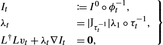
with initial and final conditions
I0=I0andλ1=−1σ2(I0∘ϕ−11−I1),
where τt≔τ(t)![]() is the flow for the negative velocity field (with τ1=Id
is the flow for the negative velocity field (with τ1=Id![]() ), and It
), and It![]() is the transformed source image at time t. The adjoint variable λ:R3×[0,1]→R
is the transformed source image at time t. The adjoint variable λ:R3×[0,1]→R![]() is initialized at t=1
is initialized at t=1![]() with the negative image mismatch (also called residual; see Section 13.3.4 on distance measures) scaled by the weighting factor 1σ2>0
with the negative image mismatch (also called residual; see Section 13.3.4 on distance measures) scaled by the weighting factor 1σ2>0![]() , which balances regularizer and distance measure energy. The spatial gradient of the image at time t is referred to as ∇It
, which balances regularizer and distance measure energy. The spatial gradient of the image at time t is referred to as ∇It![]() , and the Jacobian of the spatial variables of τ−1t
, and the Jacobian of the spatial variables of τ−1t![]() is Jτ−1t
is Jτ−1t![]() . Note that the adjoint variable λ is also called the scalar momentum in the literature [98], and the quantity λ∇I=m
. Note that the adjoint variable λ is also called the scalar momentum in the literature [98], and the quantity λ∇I=m![]() is the vector-valued momentum [90]. In fact, the optimality conditions can be written solely with respect to the vector-valued momentum m, resulting in the EPDiff equation; see, for example, [67].
is the vector-valued momentum [90]. In fact, the optimality conditions can be written solely with respect to the vector-valued momentum m, resulting in the EPDiff equation; see, for example, [67].
Computing the variation leading to (13.4) and (13.5) in the optimize–discretize framework is rather involved. If the interest is only in I1![]() , alternatively the flow equation in the form of a transport equation in Eulerian coordinates can be added as a constraint to the optimization problem. This has been proposed by Borzí et al. [8] for optical flow and by Hart et al. [45] for LDDMM. Following [45], the LDDMM formulation then becomes
, alternatively the flow equation in the form of a transport equation in Eulerian coordinates can be added as a constraint to the optimization problem. This has been proposed by Borzí et al. [8] for optical flow and by Hart et al. [45] for LDDMM. Following [45], the LDDMM formulation then becomes
EHart(v,I)=Reg(v)+SimSSD(I1,I1),s.t.˙It+∇I⊤tvt=0,I0=I0,}

with the optimality conditions
˙It+∇I⊤tvt=0,I0=I0,˙λt+div(λtvt)=0,λ1=−1σ2(I1−I1),L†Lvt+λt∇It=0.}

The optimality conditions (13.4)–(13.5) and (13.7) are the same, but (13.7) are written directly in terms of the image I and the Lagrange multiplier λ. In practice both formulations are solved by computing the flows ϕ and τ from which the solution of the transport equation (for I) can be obtained by interpolation.3 The solution for the scalar conservation law/the continuity equation for λ is obtained by interpolation and local weighting by the determinant of the Jacobian of the transformation.
The advantage of the second optimize–discretize approach (13.6) is that the optimality conditions (13.7) are (relatively) easy to derive and retain physical interpretability. For example, it is immediately apparent that the adjoint to the transport equation is a scalar conservation law. However, great care needs to be taken to make sure that all equations and their boundary conditions are consistently discretized in the optimize–discretize approach. For example, it cannot be guaranteed that for any given discretization, the gradients computed based on the discretized optimality conditions will minimize the overall energy [35]. In particular, these formulations require interpolation steps, which can cause trouble with the optimization, because it is unclear how they should affect a discretized gradient. Furthermore, the flow equations can be discretized in various ways (e.g., by a semi-Lagrangian scheme [7], upwind schemes [45], etc.). But, as these discretizations are not considered part of the optimization, their effect on the gradient remains unclear.
Therefore we follow the discretize–optimize approach in image registration [66, p. 12], which starts out with a discretization of the energy to be minimized and derives the optimality conditions from this discretized representation. Our approach is related to the work by Wirth et al. [101,83] on geodesic calculus for shapes but approaches the problem from an optimal control viewpoint.
In [5] the diffeomorphic matching is phrased as an optimal control problem, which is solved using a discretize–optimize approach. This method is related to the approach we will propose, but instead of matching images, in [5] surfaces and point clouds are registered. Another difference is the use of explicit first-order Runge–Kutta methods (i.e., forward Euler discretization), whereas we are using fourth-order methods (see Section 13.5.1) to fulfill numerical stability considerations. Recently, Mang and Ruthotto [58] also formulated LDDMM registration as an optimal control problem using a discretize–optimize approach. Specifically, they use the Gauss–Newton approach, which improves the convergence rate compared to the L-BFGS method we will apply but requires the solution of additional linear systems. However, the biggest difference between our proposed approach and the approach by Mang et al. [58] is that we use explicit Eulerian discretizations of the partial differential equation constraints of LDDMM via Runge–Kutta methods, whereas Mang et al. [58] use Lagrangian methods. Although such Lagrangian methods are attractive as they eliminate the risk of numerical instabilities and allow for arbitrary time step sizes, they require frequent interpolations and consequentially become computationally demanding. Instead, our formulation operates on a fixed grid and only requires interpolations for the computation of the image distance measure. To avoid numerical instabilities due to too large time-steps, we investigate how an admissible step size can be chosen under easily obtainable estimations for the maximal displacement when using a fourth-order Runge–Kutta method. To illustrate the difference in computational requirements, we note that although in [58] experiments were performed on a compute node with 40 CPUs, the computation for a 3D registration (with a number of voxels per image that is only about 10% of the voxel numbers of the images we are registering) takes between 25 and 120 minutes and thus is two to five times slower than our proposed methods on a single CPU. This dramatic difference in computational effort is most likely due to the tracking of the points/particles in the Lagrangian setting or the required interpolations.
An optimal solution v⁎![]() fulfills the optimality conditions (e.g., (13.7)). However, these conditions need to be determined numerically. The classical approach, proposed in [7], is the so-called relaxation approach. Here, for a given v, the transport equation for I is solved forward in time and the adjoint equation for λ backward in time. Given I and λ, the gradient of the energy with respect to the velocity v at any point in space and time can be computed, i.e.,
fulfills the optimality conditions (e.g., (13.7)). However, these conditions need to be determined numerically. The classical approach, proposed in [7], is the so-called relaxation approach. Here, for a given v, the transport equation for I is solved forward in time and the adjoint equation for λ backward in time. Given I and λ, the gradient of the energy with respect to the velocity v at any point in space and time can be computed, i.e.,
∇vtE(v,I)=L†Lvt+λt∇It,
which can then, for example, be used in a gradient descent solution scheme. In practice typically the Hilbert-gradient is used [7]
∇HvtE(v,I)=vt+(L†L)−1(λt∇It)
to improve numerical convergence.4 Upon convergence, a relaxation approach will fulfill the optimality conditions, which describe a geodesic path [7]. Unfortunately, the optimality conditions will in practice frequently not be fulfilled exactly, and the relaxation approach requires optimization over the full spatio-temporal velocity field v, whereas the geodesic path is completely specified by its initial conditions, that is, its initial velocity v0![]() and its initial image I0
and its initial image I0![]() . This has motivated the development of shooting approaches [3,98], where ones optimizes over the initial conditions of the geodesic directly instead of v. The numerical solution is similar to the relaxation approach in the sense that the adjoint system is derived to compute the gradient with respect to the initial conditions through a forward–backward sweep. Shooting approaches also allow for extensions to the LDDMM registration models, such as LDDMM-based geodesic regression [70].
. This has motivated the development of shooting approaches [3,98], where ones optimizes over the initial conditions of the geodesic directly instead of v. The numerical solution is similar to the relaxation approach in the sense that the adjoint system is derived to compute the gradient with respect to the initial conditions through a forward–backward sweep. Shooting approaches also allow for extensions to the LDDMM registration models, such as LDDMM-based geodesic regression [70].
A common problem with LDDMM is its large memory footprint and the high computational costs. For example, to register lung CT images, run times of up to three hours on a computer with 128 GB of RAM and 32 CPUs have been reported [86]. In particular, for the shooting approaches, several ideas to overcome these problems have been proposed. Marsland and McLachlan [59] and Durrleman et al. [27] use a limited number of control points for LDDMM and observe that the number of control points can be decreased substantially (i.e., much fewer control points than number of pixels or voxels are needed) without greatly impacting the registration result. Zhang et al. [107] exploit the smoothness of the velocities in the Fourier domain. The underlying idea is that the initial velocities of the geodesic shooting are band-limited and therefore can be well approximated by a limited number of elements of a finite-dimensional vector space.
In contrast to the brain MRI or synthetic examples discussed in most LDDMM publications (see, e.g., [7,27,107]), lung registration (our motivating registration application) requires aligning many small spatially distributed salient structures (such as vessels). Hence the spatial discretization for the images cannot be too coarse as it would otherwise risk ignoring these fine structures. We can still reduce computational costs and memory requirements by recognizing that velocity fields will be smooth. Specifically, as we assume that the structures of interest are well dispersed over the whole lung volume, we employ regular grids for the velocity fields (or momenta fields). However, as confirmed in our own previous work [76], velocity fields can be discretized more coarsely (about one quarter of resolution per dimension) than the images themselves due to their inherent smoothness. We thereby obtain a method that aligns images well without losing accuracy compared to higher-resolution approaches while reducing computational costs and memory requirements.
13.3 Continuous mathematical models
In this section we introduce the continuous models that will be solved in a discretize–optimize approach. Fig. 13.1 shows different options. To obtain a consistent discretization for relaxation and shooting, we would ideally like to start from a discretized LDDMM energy, derive the KKT conditions, impose the KKT conditions as a constraint, and then obtain a discretization of the shooting equations, which is consistent with the relaxation equations (i.e., the KKT equations of the discretized LDDMM energy). However, this is difficult in practice as it would no longer allow the use of explicit time-integration schemes. Instead, we suggest separate discretize–optimize approaches for the relaxation and the shooting formulations of LDDMM. For the discretize–optimize formulation of relaxation, we simply discretize the LDDMM energy including the transport equation constraint. We discuss in Section 13.3.1 the related continuous relaxation energies for the direct transport of images, whereas in Section 13.3.2 the corresponding energies for the transport of maps are considered. Alternatively, for the discretize–optimize approach for the shooting formulation of LDDMM, it is sensible to start with the discretized energy of the continuous shooting model including the associated constraints given by the EPDiff equation, which are described in Section 13.3.3.

In contrast to the methods presented in Section 13.2, we will use a general distance measure in what follows. Specifically, distance measures quantify the similarity of images by assigning a low (scalar) value to image pairs that are similar and a large value to image pairs that are different. Formally, we define the set of gray-value images as I≔{I:Ω→R}![]() . A distance measure is a mapping Sim:I×I→R
. A distance measure is a mapping Sim:I×I→R![]() [65, p. 55]. We assume that the distance measure is differentiable and that ∇ASim(A,B)
[65, p. 55]. We assume that the distance measure is differentiable and that ∇ASim(A,B)![]() is the derivative with respect to the first image. In Section 13.3.4 we give details of the used distance measures. Next, we describe the models we will use for registration. These are extensions of the methods in Section 13.2 and are called IBR, MBR, and MBS, respectively, where I means image, M map, B based, R relaxation, and S shooting.
is the derivative with respect to the first image. In Section 13.3.4 we give details of the used distance measures. Next, we describe the models we will use for registration. These are extensions of the methods in Section 13.2 and are called IBR, MBR, and MBS, respectively, where I means image, M map, B based, R relaxation, and S shooting.
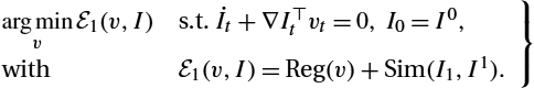
13.3.1 Relaxation with transport of images (IBR)
We extend the relaxation model of Hart et al. [45] (see (13.6)) via a general differentiable distance measure Sim. This model is a relaxation model as the optimization is performed with respect to the full spatio-temporal velocity field in t∈[0,1]![]() . This is in contrast to shooting approaches where images (or transformations) are following a flow determined completely by initial conditions at t=0
. This is in contrast to shooting approaches where images (or transformations) are following a flow determined completely by initial conditions at t=0![]() ; see Section 13.3.3. We do not explicitly model a transformation ϕ to transform the source image, but directly compute the image mismatch between the modeled image at t=1
; see Section 13.3.3. We do not explicitly model a transformation ϕ to transform the source image, but directly compute the image mismatch between the modeled image at t=1![]() (I(1)=I1
(I(1)=I1![]() ) and the target image I1∈I
) and the target image I1∈I![]() :
:
argminvE1(v,I)s.t.˙It+∇I⊤tvt=0,I0=I0,withE1(v,I)=Reg(v)+Sim(I1,I1).}
13.3.2 Relaxation with transport of maps (MBR)
Typically, the spatial transform ϕ is of interest and needs to be computed, for example, to calculate local volume changes during respiration [95]. This transform can be computed via time-integration of the spatio-temporal velocity field. Hence, in Eulerian coordinates we now advect a deformation map instead of an image. When solving the transport equation this is advantageous because the deformations are smooth by design and thus suffer less from dissipation effects than images.
As our goal is to work with fixed computational grids (i.e., in Eulerian coordinates), we can also write the evolution equation for the inverse map ϕ−11![]() in Eulerian coordinates. The inverse transformation ϕ−11
in Eulerian coordinates. The inverse transformation ϕ−11![]() is required to deform the source image to the coordinate system of the target image (i.e., I0∘ϕ−11
is required to deform the source image to the coordinate system of the target image (i.e., I0∘ϕ−11![]() ; see (13.1)).
; see (13.1)).
The evolution of ϕ−11![]() is given by [63].
is given by [63].
˙ϕ−1t=−Jϕ−1tvt,ϕ0−1=Id,
which is nothing else than a set of independent transport equations for the coordinate functions (x, y, and z in 3D). Here, we use the spatial Jacobian (Jϕ≔Jϕ(x,t)∈R3×3![]() ) of ϕ=(ϕ1,ϕ2,ϕ3)⊤
) of ϕ=(ϕ1,ϕ2,ϕ3)⊤![]() , which is defined as
, which is defined as
Jϕ≔(∂x1ϕ1t(x)∂x2ϕt1(x)∂x3ϕ1t(x)∂x1ϕ2t(x)∂x2ϕ2t(x)∂x3ϕ2t(x)∂x1ϕ3t(x)∂x2ϕ3t(x)∂x3ϕ3t(x)).

Note, that we used superscripts to refer to the components of vectors such as ϕ(x,t)∈R3![]() . As the point of view for the time direction of the transformations is arbitrary, we change the notation of the inverse transformation used in [7] (see also (13.1)) for convenience to ϕ. This results in the simplified notation
. As the point of view for the time direction of the transformations is arbitrary, we change the notation of the inverse transformation used in [7] (see also (13.1)) for convenience to ϕ. This results in the simplified notation
˙ϕt+Jϕtvt=0,ϕ0=Id.
We use (13.13) as the constraint for the map-based optimization problem:
argminvE2(ϕ,v)s.t. ˙ϕt+Jϕtvt=0,ϕ0=Id,withE2(ϕ,v)≔Reg(v)+Sim(I0∘ϕ1,I1).}

13.3.3 Shooting with maps using EPDiff (MBS)
Recall that the optimality conditions of the relaxation formulation can be written with respect to the vector-valued momentum m only. Hence, instead of obtaining a solution to these optimality conditions at convergence (as done in the relaxation approach), we simply enforce these optimality conditions as constraints in an optimization problem. This is the shooting approach [62,98]. Specifically, if we express these conditions with respect to the momentum, then we obtain the EPDiff equation (abbreviation for the Euler–Poincaré equation on the group of diffeomorphisms) [47,61,105]
˙mt=−Jmtvt−mtdiv(vt)−J⊤vtmt,vt=Kmt.
Here m:Ω×[0,1]→R3![]() is the momentum, and K=(L†L)−1
is the momentum, and K=(L†L)−1![]() is a smoothing kernel. This equation describes a geodesic path and fully determines the transformation as it implies an evolution of the velocities v via vt=Kmt
is a smoothing kernel. This equation describes a geodesic path and fully determines the transformation as it implies an evolution of the velocities v via vt=Kmt![]() . The total momentum will be constant for a geodesic due to the conservation of momentum [104,98]:
. The total momentum will be constant for a geodesic due to the conservation of momentum [104,98]:
〈Km0,m0〉=〈Kmt,mt〉,t∈[0,1].
If we integrate (13.15) and (13.16) into (13.14), then the minimization problem has the following form:
argminm0E3(m,ϕ,v)s.t.∂tϕ+Jϕv=0,ϕ0=Id,∂tm+Jmv+mdiv(v)+J⊤vm=0,v=Km,with E3≔121∫0〈mt,Kmt〉dt+Sim(I0∘ϕ1,I1)(13.16)=12〈m0,Km0〉+Sim(I0∘ϕ1,I1).}

13.3.4 Distance measures
Registration quality depends on the appropriateness of the deformation model and the distance measure. Different distance measures can easily be integrated into LDDMM; see [22,4]. Note that we formulate our models in generality and that the following derivations hold for a large class of differentiable distance measures [66, p. 109]:
Sim(A,B)≔1σ2ψ(r(A,B)),
where r is the residuum or image mismatch of A and B, and ψ is typically an integral of the residual values. The functions r and ψ are assumed to be at least once differentiable. This is necessary to allow derivative-based optimization, which we are using in our discretize–optimize schemes. Data fidelity and regularity are balanced via the weight σ>0![]() , which can be interpreted as the image noise level. We use two different differentiable distance measures in our experiments. The L2
, which can be interpreted as the image noise level. We use two different differentiable distance measures in our experiments. The L2![]() -based distance measure sum of squared differences (SSD) [65, p. 56] is used in most LDDMM publications (see, e.g., [7,45,107]):
-based distance measure sum of squared differences (SSD) [65, p. 56] is used in most LDDMM publications (see, e.g., [7,45,107]):
SimSSD(A,B)=12σ2∫Ω(A(x))−B(x))2dx.

Hence ψSSD(r)=12∫Ωr(x)2dx![]() , and the residuum is the difference rSSD(A,B)=A−B
, and the residuum is the difference rSSD(A,B)=A−B![]() . As motivated in Section 13.1, we will use the normalized gradient field (NGF) distance measure for the registration of lung CT images. NGF aligns image edges [38,66] and is popular for lung CT registration [81,51,74–76]:
. As motivated in Section 13.1, we will use the normalized gradient field (NGF) distance measure for the registration of lung CT images. NGF aligns image edges [38,66] and is popular for lung CT registration [81,51,74–76]:
SimNGF(A,B)≔1σ2∫Ω1−〈∇A,∇B〉2ε‖∇A‖2ε‖∇B‖2εdx

with 〈u,v〉ε≔ε2+∑3i=1uivi![]() and ‖u‖2ε≔〈u,u〉ε
and ‖u‖2ε≔〈u,u〉ε![]() for u, v∈R3
for u, v∈R3![]() . Throughout this chapter we set ε=50
. Throughout this chapter we set ε=50![]() for lung CT registrations. Rewriting SimNGF
for lung CT registrations. Rewriting SimNGF![]() with ψ and r yields:
with ψ and r yields:
ψNGF(r)=∫Ω1−r(x)2dx,rNGF(A,B)=〈∇A,∇B〉ε‖∇A‖ε‖∇B‖ε.

This concludes the description of the continuous LDDMM models. In the following sections we present their discretization.
13.4 Discretization of the energies
In this section we describe the numerical computation of the continuous energies introduced in Section 13.3. We start with the description of the different regular grids, which are used for discretization of the velocities, images, transformations, et cetera in Section 13.4.1. The discretization of the regularizer and the distance measures is addressed in Section 13.4.2 and Section 13.4.3 respectively.
13.4.1 Discretization on grids
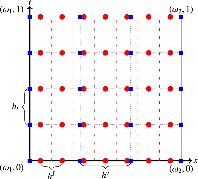
We use regular grids to discretize v, I, ϕ, et cetera in time and space. To properly handle boundary conditions, it is important to discuss on which grid the velocities and images are given. In particular, we choose nodal grids for the velocities v and transformations ϕ and cell-centered grids for the images I. For simplicity, we start with the discretization for the one-dimensional space. We assume that the discrete source and target images have M∈N![]() values located at equidistant centers of intervals whose union is the closure of the domain ˉΩ=[ω1,ω2]⊂R
values located at equidistant centers of intervals whose union is the closure of the domain ˉΩ=[ω1,ω2]⊂R![]() . For the nodal grids n∈N
. For the nodal grids n∈N![]() , n⩾2
, n⩾2![]() points are used. Details on both types of grids are given, for example, in [66, p. 125].
points are used. Details on both types of grids are given, for example, in [66, p. 125].
Fig. 13.2 shows two example grids. The nodal grid is depicted as blue (dark gray in print version) squares, whereas the cell-centered grid is visualized as red (light gray in print version) dots. Note that the number of cells for images and velocities does not need to be equal. In fact, it is the key idea of our approach to speed up computations and reduce memory requirements by discretizing velocity and transformation fields on a lower resolution grid than the images, that is, n<M![]() . Consequently, we have different spatial step sizes hv1≔ω2−ω1n−1
. Consequently, we have different spatial step sizes hv1≔ω2−ω1n−1![]() and hI1≔ω2−ω1M
and hI1≔ω2−ω1M![]() . As we consider only one dimension first, we will omit the indices and write hv
. As we consider only one dimension first, we will omit the indices and write hv![]() and hI
and hI![]() . The time axis [0,1]
. The time axis [0,1]![]() is discretized for v, ϕ, and I on a nodal grid with N time steps, and accordingly the time step size is ht≔1N−1
is discretized for v, ϕ, and I on a nodal grid with N time steps, and accordingly the time step size is ht≔1N−1![]() . The resulting nodal grid is xnd∈RnN
. The resulting nodal grid is xnd∈RnN![]() , and the cell-centered image grid is a vector xcc∈RMN
, and the cell-centered image grid is a vector xcc∈RMN![]() . The discretized velocity field is then given as v≔v(xnd)∈Rn×N
. The discretized velocity field is then given as v≔v(xnd)∈Rn×N![]() . Accordingly, the images are discretized as I≔I(xcc)∈RM×N
. Accordingly, the images are discretized as I≔I(xcc)∈RM×N![]() .
.
When solving the constraint equations (e.g., the transport equation for images in (13.10)), we need images and velocities discretized at the same resolution. We therefore use a linear grid interpolation (bi/trilinear for 2D/3D data). The appropriate weights are stored in the components of the interpolation matrix P∈RM×n![]() . See [51,80] on how to compute the weights and how to implement a matrix-free computation of the matrix–matrix product. By multiplying the velocity matrix v with the matrix P we obtain a cell-centered discretization Pv∈RM×N
. See [51,80] on how to compute the weights and how to implement a matrix-free computation of the matrix–matrix product. By multiplying the velocity matrix v with the matrix P we obtain a cell-centered discretization Pv∈RM×N![]() , which can be used to transport the intensities located at the image grid points. When solving the adjoint equation of, for example, (13.7), the transposed matrix has to be used to interpolate the derivative of the distance measure to the nodal grid to update the velocities.
, which can be used to transport the intensities located at the image grid points. When solving the adjoint equation of, for example, (13.7), the transposed matrix has to be used to interpolate the derivative of the distance measure to the nodal grid to update the velocities.
13.4.2 Discretization of the regularizer
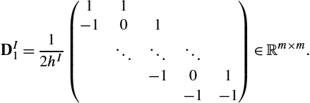
Two main computations are required to discretize the regularization term. First, we compute the differential operator L, which is based on second derivatives, and its effect on the velocity field to be regularized. Second, we approximate the integral of the regularizer using numerical quadrature. In particular, we use the trapezoidal rule. Here we formulate everything initially in 1D for simplicity and assume Neumann boundary conditions for the velocities v and Dirichlet boundary conditions for the images throughout. The discretized regularizer has the form
Regh(ˉv)≔hvht2ˉv⊤ˉL⊤WˉLˉv,
and we proceed with details on the computation of ˉL![]() , ˉv
, ˉv![]() , and W.
, and W.
We use a standard approach to discretize the Helmholtz operator L=(γId−αΔ)β![]() with Neumann boundary conditions; see, for example, [92]. The derivatives are approximated with central finite differences. The proper choice of the parameters α, γ>0
with Neumann boundary conditions; see, for example, [92]. The derivatives are approximated with central finite differences. The proper choice of the parameters α, γ>0![]() and β∈N
and β∈N![]() depends on the application and in particular on the spatial dimension k∈N
depends on the application and in particular on the spatial dimension k∈N![]() . For instance, to obtain diffeomorphic solutions for k=3
. For instance, to obtain diffeomorphic solutions for k=3![]() , at least β=2
, at least β=2![]() is needed [26]. To be more precise, using Sobolev embedding theorems [108, p. 62], the following inequality has to be fulfilled (see [60] and references therein):
is needed [26]. To be more precise, using Sobolev embedding theorems [108, p. 62], the following inequality has to be fulfilled (see [60] and references therein):
s>k2+1,
where s is the order of the Hs![]() metric used for the velocity fields vt
metric used for the velocity fields vt![]() , t∈[0,1]
, t∈[0,1]![]() . For v∈Rn×N
. For v∈Rn×N![]() , the discrete operator is L∈Rn×n
, the discrete operator is L∈Rn×n![]() :
:
L≔(γIdn−αΔhv)β,
where Idn∈Rn×n![]() is the identity matrix, and
is the identity matrix, and
Δhv≔1(hv)2(−111−21⋱⋱⋱1−211−1)
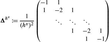
is a discrete Laplacian operator. We use a trapezoidal quadrature for integration in space and time. The different weights for inner and outer grid points are assigned by multiplication with the diagonal matrix W∈RnN×nN![]() . Kronecker products are used for a compact notation and to compute ˉL∈RnN×nN
. Kronecker products are used for a compact notation and to compute ˉL∈RnN×nN![]() , which enables regularization for all time steps at once:
, which enables regularization for all time steps at once:
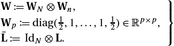
W≔WN⊗Wn,Wp≔diag(12,1,…,1,12)∈Rp×p,ˉL≔IdN⊗L.}
If we use the column-vector representation of v,
ˉv≔(v1,1,…,vn,1,v1,2,…,vn,2,…,v1,N,…,vn,N)⊤,
and (13.25), then we obtain (13.21) for the discretized regularizer.
13.4.3 Discretization of the distance measures
For simplicity, we only give details of the discretization of the SSD distance measure defined in (13.19). For two discrete one-dimensional images A=(ai)Mi=1![]() and B=(bi)Mi=1
and B=(bi)Mi=1![]() (e.g., the discrete source (I0
(e.g., the discrete source (I0![]() ) and target (I1
) and target (I1![]() ) images), we use a midpoint quadrature to compute the discrete distance measure value
) images), we use a midpoint quadrature to compute the discrete distance measure value
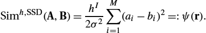
Simh,SSD(A,B)=hI2σ2M∑i=1(ai−bi)2=:ψ(r).
Hence the discrete residual for SSD is r≔r(A,B)=(ai−bi)Mi=1![]() , and the discrete outer function is given as ψ(r)=hI2σ2∑Mi=1r2i
, and the discrete outer function is given as ψ(r)=hI2σ2∑Mi=1r2i![]() . The numerical gradient, which will be needed for numerical optimization, consists of the following derivatives:
. The numerical gradient, which will be needed for numerical optimization, consists of the following derivatives:
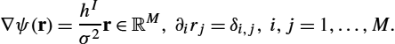
∇ψ(r)=hIσ2r∈RM,∂irj=δi,j,i,j=1,…,M.
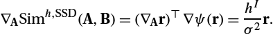
Hence the numerical Jacobian of r is just the identity matrix, ∇Ar=IdM∈RM×M![]() . Based on these results, (13.27), and the chain rule, we obtain the numerical gradient for the distance measure:
. Based on these results, (13.27), and the chain rule, we obtain the numerical gradient for the distance measure:
∇ASimh,SSD(A,B)=(∇Ar)⊤∇ψ(r)=hIσ2r.
We transposed the inner and outer derivative in (13.28) as we assume column vector gradients throughout the chapter. For discretizations of SSD in multiple dimensions or other distance measures, such as NGF, we refer to [66, p. 107].
13.5 Discretization and solution of PDEs
The partial differential equations we need to solve are the transport/advection equation, the EPDiff equation, and the adjoint equations of the models (13.10), (13.14), and (13.17).
The standard LDDMM registrations use semi-Lagrangian methods [7] or upwinding for the solution of the transport equation [45]. In this work semi-Lagrangian methods are not used as they require interpolations at every time step and hence have substantially increased computational costs. Upwinding includes logical switches, which interfere with our model, which requires differentiable constraints. We therefore focus on methods that use central differences to compute spatial derivatives. However, this then requires appropriate schemes for time-integration as, for example, an Euler forward scheme, which is known to be unconditionally unstable in such a case [92] for the solution of the transport equation. An implicit scheme generates stable solutions, but solving many linear equation systems is too expensive for our image registration purposes. As a compromise, we use explicit fourth-order Runge–Kutta methods, which have a sufficiently large stability region (and in particular include part of the imaginary axis) and have acceptable computational requirements; see Section 13.5.1. In Section 13.5.2 we describe how to consistently solve the adjoint equations (e.g., scalar conservation/continuity equations). We then apply these approaches to the IBR (Section 13.5.3), MBR (Section 13.5.4), and MBS (Section 13.5.5) models.
First, consider the one-dimensional transport equation, which is part of the IBR model:
˙It+(∂xIt)vt=0,I0=I0.
The spatial derivative is approximated with central finite differences and homogeneous Dirichlet boundary conditions are assumed for the images. The matrix to compute the discrete image derivatives is
DI1=12hI(11−101⋱⋱⋱−101−1−1)∈Rm×m.
For tℓ=ℓht∈[0,1]![]() , ℓ=0,…,N−1
, ℓ=0,…,N−1![]() , we approximate the spatial derivative for all image grid points xcc
, we approximate the spatial derivative for all image grid points xcc![]() as
as
∂xI(xcc,tℓ)≈DI1Iℓ,
where Iℓ![]() is the (ℓ+1)
is the (ℓ+1)![]() th column of I, that is, the image at time tℓ
th column of I, that is, the image at time tℓ![]() .
.
13.5.1 Runge–Kutta methods
In the following we will use notation that is common in optimal control publications. In particular, x is not a spatial variable, but it is the state we are interested in, for example, an evolving image or transformation map. Solving the transport equation (13.29) is an initial value problem of the form
˙x(t)=f(x(t),u(t)),x0≔x(0)=x0,t∈[0,1],
where x(t)∈Rp![]() with initial value x0=x0∈Rp
with initial value x0=x0∈Rp![]() is the state variable, and u(t)∈Rq
is the state variable, and u(t)∈Rq![]() is an external input called control. The change over time is governed by the right-hand side function f:Rp×Rq→Rp
is an external input called control. The change over time is governed by the right-hand side function f:Rp×Rq→Rp![]() .
.
To avoid excessive smoothing when solving (13.29) numerically, we do not use methods that introduce additional diffusion to ensure stability for the Euler forward method such as Lax–Friedrichs [92]. Instead, we use a Runge–Kutta method, which includes at least part of the imaginary axis in its stability region. We can then discretize the spatial derivative of the transport equation using central differences as given in (13.30) and (13.31) while still maintaining numerical stability.
Runge–Kutta methods have been investigated in the context of optimal control, for example, by Hager [39,40]. Since we are dealing with a Hamiltonian system, we would ideally like to pick a symplectic Runge–Kutta scheme [43, p. 179] as proposed for image registration in [59]. Consistent approximations have been explored in [89]. In particular, we are interested in a symplectic symmetric Runge–Kutta scheme [20], which preserves the energy of the system (here the Sobolev norm of the velocity) [85]. Energy-preserving Runge–Kutta methods have been investigated in [19]. The simplest such method is the implicit midpoint method [59,19]. However, implicit Runge–Kutta methods require the solution of an equation system at every iteration step. Although this can be accomplished by Newton's method or a fixed point iteration, it may compromise the symplectic property [93] and can become computationally costly.
We therefore restrict ourselves to explicit Runge–Kutta methods, which are nonsymplectic, but easy to implement, fast, and (at sufficiently high order) are only mildly dissipative and hence, experimentally, do not lose a significant amount of energy for the short time-periods we are integrating over for image registration.
We restrict the discussion to Runge–Kutta methods with s∈N![]() stages. See [42, p. 132] for details. In the general case considered now, f has an explicit time dependence f:[0,1]×Rp×Rq→Rp
stages. See [42, p. 132] for details. In the general case considered now, f has an explicit time dependence f:[0,1]×Rp×Rq→Rp![]() . Given the state variable x0=x(t0)=x0∈Rp
. Given the state variable x0=x(t0)=x0∈Rp![]() with tℓ≔ℓN−1=ℓht
with tℓ≔ℓN−1=ℓht![]() and the control uiℓ∈Rq
and the control uiℓ∈Rq![]() , ℓ=0
, ℓ=0![]() , 1,…,N−1
, 1,…,N−1![]() , i=1,…,s
, i=1,…,s![]() , the evolution of the state over time (xℓ
, the evolution of the state over time (xℓ![]() , ℓ=1,…,N−1
, ℓ=1,…,N−1![]() ) is computed with these methods.
) is computed with these methods.
One-step Runge–Kutta methods can be written as [42, p. 134]
yiℓ=xℓ+ht∑sj=1aijf(tℓ+cjht,yjℓ,ujℓ)xℓ+1=xℓ+ht∑si=1bif(tℓ+ciht,yiℓ,uiℓ),i=1,…,s,ℓ=0,…,N−2.}

According to (13.32) and our definition of f, xℓ+1≈x(tℓ+1)![]() is the approximated state, yiℓ≈x(tℓ+ciht)
is the approximated state, yiℓ≈x(tℓ+ciht)![]() are the intermediate discrete states, and uiℓ≔u(tℓ+ciht)
are the intermediate discrete states, and uiℓ≔u(tℓ+ciht)![]() are the given discrete control variables. The matrix A∈Rs×s
are the given discrete control variables. The matrix A∈Rs×s![]() and the vectors c, b∈Rs
and the vectors c, b∈Rs![]() depend on the chosen Runge–Kutta method. If c1=0
depend on the chosen Runge–Kutta method. If c1=0![]() and A is lower triangular, then the Runge–Kutta method is explicit; otherwise, it is implicit [14, p. 98]. In Table 13.1, A, b, and c are given in the so-called Butcher tableau for the fourth-order Runge–Kutta methods used for solving the state and adjoint equations in this work.
and A is lower triangular, then the Runge–Kutta method is explicit; otherwise, it is implicit [14, p. 98]. In Table 13.1, A, b, and c are given in the so-called Butcher tableau for the fourth-order Runge–Kutta methods used for solving the state and adjoint equations in this work.
Table 13.1
Butcher tableaux of the fourth-order explicit Runge–Kutta methods used in this chapter. For the adjoint system, the matrix ˉA![]() with ˉaij=bjajibi
with ˉaij=bjajibi![]() , i,j = 1,…,s, is given.
, i,j = 1,…,s, is given.
| General Butcher tableau | Runge–Kutta 4 | Adjoint Runge–Kutta 4 | ||||||||||||||||||||||||||||||||||||||||||||||||||||||
|---|---|---|---|---|---|---|---|---|---|---|---|---|---|---|---|---|---|---|---|---|---|---|---|---|---|---|---|---|---|---|---|---|---|---|---|---|---|---|---|---|---|---|---|---|---|---|---|---|---|---|---|---|---|---|---|---|
|
|
|

Because all considered constraints can be written in the form of (13.32) and thus do not have an explicit dependence on time, we can simplify (13.33) to
yiℓ=xℓ+ht∑sj=1aijf(yjℓ,ujℓ),xℓ+1=xℓ+ht∑si=1bif(yiℓ,uiℓ),i=1,…,s,ℓ=0,…,N−2.}

13.5.2 Runge–Kutta methods for the adjoint system
As mentioned before, a consistent discretization of the energies and constraints is desirable. Therefore when using Runge–Kutta integrations for time-dependent constraints, we need to compute the adjoint model of the chosen Runge–Kutta integrator. This was worked out by [40]. For completeness, we give the result using our notation. Note that the optimal control problems for the relaxation approaches considered in this chapter are Bolza problems of the form
argminx(1),uEB(x(1),u)s.t. ˙x(t)=f(x,u),x(0)=x0=x0,EB(x(1),u)≔C1(x(1))+∫10C2(x(t),u(t))dt.}

Here C1:Rp→R![]() is only depending on the final state (corresponding to the distance measure in the image registration), and C2:Rp×Rq→R
is only depending on the final state (corresponding to the distance measure in the image registration), and C2:Rp×Rq→R![]() is a cost function depending on all intermediate states and controls (which is the regularization part in LDDMM). In [40] Mayer problems with
is a cost function depending on all intermediate states and controls (which is the regularization part in LDDMM). In [40] Mayer problems with
argminx(1)EM(x(1))s.t. ˙x(t)=f(x,u),x0=x(0)=x0}

are solved. Mayer and Bolza problems are equivalent as they can be converted into each other [25, p. 159], and hence the results of Hager still apply to our problems. For the sake of a compact notation, we omit the superscripts M and B. Next, we briefly summarize how to obtain the adjoint equations of (13.35); for a complete derivation, see [40].
We introduce the arrays
X≔(xℓ)N−1ℓ=0∈Rp×N,Y≔(yiℓ)N−1,sℓ=0,i=1∈Rp×N×s,U≔(uiℓ)N−1,sℓ=0,i=1∈Rq×N×s,

which contain all discrete states, intermediate states, and control variables. Following [40] and given the discretized energy E(xN−1,U)![]() , Eqs. (13.34) are added as constraints through the Lagrangian multipliers
, Eqs. (13.34) are added as constraints through the Lagrangian multipliers
Λ≔(λℓ)N−1ℓ=1∈Rp×N−1 and Ξ≔(ξiℓ)N−2,sℓ=0,i=1,
yielding the Lagrange function
L(X,Y,U,Λ,Ξ)=E(xN−1,U)+N−2∑ℓ=0[λ⊤ℓ+1(xℓ+1−xℓ−hts∑i=1bif(yiℓ,uiℓ))+s∑i=1(ξiℓ)⊤(yiℓ−xℓ−hts∑j=1ai,jf(yjℓ,ujℓ))].}

By computing the partial derivatives of (13.37) with respect to xℓ![]() , yiℓ
, yiℓ![]() , and uiℓ
, and uiℓ![]() and substituting
and substituting
χiℓ=λℓ+1+s∑j=1ajibiξjℓ,
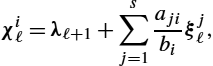
we obtain after some algebra the adjoint system and the gradient with respect to uiℓ![]() as [40]
as [40]
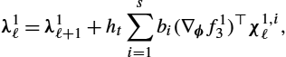
λN−1=−∇xE(xN−1,U),χiℓ=λℓ+1+hts∑j=1bjajibi(∇xf(yjℓ,ujℓ))⊤χjℓ,λℓ=λℓ+1+hts∑i=1bi(∇xf(yiℓ,uiℓ))⊤χiℓ,∇uiℓL=∇uiℓE−ht(∇uf(yiℓ,uiℓ))⊤χiℓ.}

In the case of shooting with the EPDiff equation everything is determined by the initial momentum. Hence the derivatives with respect to x0![]() of (13.37) also involve the derivative of E. The partial derivative of (13.37) with respect to the initial condition x0
of (13.37) also involve the derivative of E. The partial derivative of (13.37) with respect to the initial condition x0![]() can be shown to be
can be shown to be
∂L∂x0=∂E∂x0−λ1−hts∑i=1bi(∇xf(yi0,ui0))⊤χi0.
The latter part is (formally) the negative of the adjoint variable λ evaluated for ℓ=0![]() :
:
∂L∂x0=∂E∂x0−λ0.

Note that λℓ![]() is strictly only defined for ℓ=1,…,N−1
is strictly only defined for ℓ=1,…,N−1![]() and λ0
and λ0![]() is simply a convenience notation. The adjoint equations given in (13.39) represent a Runge–Kutta method with b and c unchanged and ‾aij=bjajibi
is simply a convenience notation. The adjoint equations given in (13.39) represent a Runge–Kutta method with b and c unchanged and ‾aij=bjajibi![]() . In particular, this implies that an explicit (implicit) Runge–Kutta method yields an explicit (implicit) Runge–Kutta method for the adjoint equations (with time reversed). The adjoint of the considered Runge–Kutta method is also shown in Table 13.1. When applied in reverse time direction, it is identical to the Runge–Kutta method used for the numerical integration of the state. Next, we will explicitly compute the equations for the 1D LDDMM registration using a transport equation on the images (i.e., the IBR model).
. In particular, this implies that an explicit (implicit) Runge–Kutta method yields an explicit (implicit) Runge–Kutta method for the adjoint equations (with time reversed). The adjoint of the considered Runge–Kutta method is also shown in Table 13.1. When applied in reverse time direction, it is identical to the Runge–Kutta method used for the numerical integration of the state. Next, we will explicitly compute the equations for the 1D LDDMM registration using a transport equation on the images (i.e., the IBR model).
13.5.3 Application to the IBR model
The states we are interested in are the discrete images X=I∈Rm×N![]() . The control sequence that influences the image transport is the velocity matrix U=v∈Rn×N
. The control sequence that influences the image transport is the velocity matrix U=v∈Rn×N![]() .
.
For the three-dimensional registration problems we are addressing later, memory consumption cannot be neglected. We therefore propose reducing the number of stored control variables uiℓ![]() . We found empirically that ‖vℓ−vℓ+1‖/‖vℓ‖
. We found empirically that ‖vℓ−vℓ+1‖/‖vℓ‖![]() for all ℓ=0,…,N−2
for all ℓ=0,…,N−2![]() was small, that is, the velocities v only change marginally over time. Hence we approximate the velocity fields within one Runge–Kutta step as piecewise constant: uiℓ≈u1ℓ=:uℓ
was small, that is, the velocities v only change marginally over time. Hence we approximate the velocity fields within one Runge–Kutta step as piecewise constant: uiℓ≈u1ℓ=:uℓ![]() , i=2,…,s
, i=2,…,s![]() . This is similar to the classical relaxation approach by Beg et al. [7], where velocities within a time-step are also assumed to be constant, and maps are then computed via a semi-Lagrangian scheme based on these constant velocity fields. Assuming piecewise constant velocity fields for our approach reduces the memory requirement for storing the control variables in U by a factor s. Empirically, this does not affect the results greatly and still constitutes a possible discretization choice for our discretize–optimize approach. Memory requirements are reduced further by the fact that the update in the last equation of (13.39) now only needs to be computed for one instead of s controls for each time tℓ
. This is similar to the classical relaxation approach by Beg et al. [7], where velocities within a time-step are also assumed to be constant, and maps are then computed via a semi-Lagrangian scheme based on these constant velocity fields. Assuming piecewise constant velocity fields for our approach reduces the memory requirement for storing the control variables in U by a factor s. Empirically, this does not affect the results greatly and still constitutes a possible discretization choice for our discretize–optimize approach. Memory requirements are reduced further by the fact that the update in the last equation of (13.39) now only needs to be computed for one instead of s controls for each time tℓ![]() . Additionally, the χiℓ
. Additionally, the χiℓ![]() are then only needed in the update for λℓ
are then only needed in the update for λℓ![]() and do not have to be stored for later computations to update the controls as χ1ℓ=λℓ
and do not have to be stored for later computations to update the controls as χ1ℓ=λℓ![]() for the explicit methods considered for numerical integration.
for the explicit methods considered for numerical integration.
As motivated in Section 13.4.1, n and m might be different, and we use the interpolation matrix P to change from the v given on a nodal grid to the resolution of I that is given on a cell-centered grid. The right-hand side function for our Runge–Kutta method then follows from (13.29) to (13.31):
f1(Iℓ,vℓ)≔−diag(DI1Iℓ)Pvℓ=−(DI1Iℓ)⊙(Pvℓ),
where ⊙ denotes the Hadamard product. The resulting derivatives needed are:
∇Iℓf1(Iℓ,vℓ)=−diag(Pvℓ)DI1,
∇vℓf1(Iℓ,vℓ)=−diag(DI1Iℓ)P.
The concrete Bolza energy (13.35), that is, the discretized objective function of (13.10), for our problem is given as
E1(IN−1,v)≔Regh(ˉv)+Simh(IN−1,I1).
Taking a closer look at (13.21), we easily compute
∇vE1(IN−1,v)=hvhtˉLWˉLˉv.
For the update of vℓ![]() , ℓ=0,…,N−1
, ℓ=0,…,N−1![]() , the components ℓn+1,…,(ℓ+1)n
, the components ℓn+1,…,(ℓ+1)n![]() of ∇vE1(IN−1,v)
of ∇vE1(IN−1,v)![]() have to be used.
have to be used.
To compute the final adjoint state λN−1∈Rm![]() , the derivative of the discrete distance measure is needed:
, the derivative of the discrete distance measure is needed:
λN−1=−∇ASimh(IN−1,I1),
where ∇ASimh![]() denotes the derivative with respect to the first argument of Simh
denotes the derivative with respect to the first argument of Simh![]() .
.
13.5.4 Application to the MBR model
As a smooth transition at the boundary of the domain is expected for the transformations, we assume homogeneous Neumann boundary conditions. The corresponding matrix to compute the discrete derivative for one component of the transformations given on a nodal grid is
Dv1=12hv(00−101⋱⋱⋱−10100)∈Rn×n.

The discrete transformation maps ϕ≔ϕ(xnd)∈Rn×N![]() are discretized exactly like the velocities. As before, ϕℓ
are discretized exactly like the velocities. As before, ϕℓ![]() is the (ℓ+1)
is the (ℓ+1)![]() th column of ϕ and ℓ∈{0,1,…,N−1}
th column of ϕ and ℓ∈{0,1,…,N−1}![]() . To include the full information provided by the images, we will interpolate I0
. To include the full information provided by the images, we will interpolate I0![]() linearly using PϕN−1
linearly using PϕN−1![]() and write ˜I0≔I0∘(PϕN−1)
and write ˜I0≔I0∘(PϕN−1)![]() for the resulting image. The discretized objective function of (13.14) then has the following form:
for the resulting image. The discretized objective function of (13.14) then has the following form:
E2(ϕN−1,v)=Regh(ˉv)+Simh(˜I0,I1).
Prolongating ϕN−1![]() with P also has an impact on the size of the adjoint variable λ∈Rm×N
with P also has an impact on the size of the adjoint variable λ∈Rm×N![]() , and the final state is
, and the final state is
λN−1=−ddPϕN−1Simh(˜I0,I1)=−∇ASimh(˜I0,I1)∇h˜I0.

For the second equation, the chain rule was applied yielding the product of the discrete gradient ∇h˜I0∈Rm![]() and ∇ASimh
and ∇ASimh![]() .
.
The discrete right-hand side function f2![]() for the transport of the transformation maps is almost identical to (13.42), only the discrete derivatives are changed, and no interpolation is needed:
for the transport of the transformation maps is almost identical to (13.42), only the discrete derivatives are changed, and no interpolation is needed:
f2(ϕℓ,vℓ)=−diag(Dv1ϕℓ)vℓ=−(Dv1ϕℓ)⊙vℓ.
The derivatives of (13.51) needed for computing the adjoint equations are:
∇ϕℓf2(ϕℓ,vℓ)=−diag(vℓ)Dv1,
∇vℓf2(ϕℓ,vℓ)=−diag(Dv1ϕℓ).
The regularization, which depends on the control variable, in this model (13.49) is the same as (13.45), and hence the partial derivative is equal to (13.46). However, the distance measure depends on the interpolated image I0(PϕN−1)![]() , and it is possible that ϕN−1
, and it is possible that ϕN−1![]() has a lower resolution than I0
has a lower resolution than I0![]() . Because the high resolution of the image mismatch (this is essentially the role of the adjoint λ) should be retained during the solution of the adjoint equations, the matrix P is used to connect Eqs. (13.52) and (13.53) to (13.50). The evolution of λ backward in time is then determined by (13.43) instead of (13.52). Also, before using λ to compute the update for the control v using (13.53), the grid change has to be undone by computing P⊤λ
. Because the high resolution of the image mismatch (this is essentially the role of the adjoint λ) should be retained during the solution of the adjoint equations, the matrix P is used to connect Eqs. (13.52) and (13.53) to (13.50). The evolution of λ backward in time is then determined by (13.43) instead of (13.52). Also, before using λ to compute the update for the control v using (13.53), the grid change has to be undone by computing P⊤λ![]() . By doing computations stepwise (i.e., storing only λℓ
. By doing computations stepwise (i.e., storing only λℓ![]() and λℓ−1
and λℓ−1![]() on the high image resolution, ℓ=1,…,N−1
on the high image resolution, ℓ=1,…,N−1![]() ) and keeping the shorter vectors P⊤λℓ
) and keeping the shorter vectors P⊤λℓ![]() the memory requirements can be reduced.
the memory requirements can be reduced.
13.5.5 Application to the MBS model using EPDiff
We briefly repeat the constraints of the MBS model:
˙ϕt+J⊤ϕtvt=0,ϕ0=Id,
˙mt+Jmtvt+mtdiv(vt)+J⊤vtmt=0,
vt=Kmt,K=(L†L)−1.
How (13.54) is solved numerically is described in Section 13.5.4. In 1D the EPDiff equation (13.55) simplifies to
˙mt+(∂xmt)vt+2mt(∂xvt)=0.
Because of (13.56), the momentum m is discretized on the same grid as the velocities. Hence our discrete representation is given on the nodal grid xnd![]() : m=m(xnd)∈Rn×N
: m=m(xnd)∈Rn×N![]() , and the matrix Dv1
, and the matrix Dv1![]() is also used for numerical derivation of the momentum.
is also used for numerical derivation of the momentum.
The adjoint of the discrete differential operator L defined in (13.23) is the transposed matrix L⊤![]() . As L is symmetric, L=L⊤
. As L is symmetric, L=L⊤![]() . Furthermore, for a positive weight γ, the matrix L is positive definite, and we can deduce that L⊤L
. Furthermore, for a positive weight γ, the matrix L is positive definite, and we can deduce that L⊤L![]() is invertible. We can deduce that the kernel K≔(L⊤L)−1∈Rn×n
is invertible. We can deduce that the kernel K≔(L⊤L)−1∈Rn×n![]() is positive definite and (13.56) can be discretized as vℓ=Kmℓ
is positive definite and (13.56) can be discretized as vℓ=Kmℓ![]() . Due to the positive definiteness of K, the latter equation system has a unique solution for all ℓ∈{0,…,N−1}
. Due to the positive definiteness of K, the latter equation system has a unique solution for all ℓ∈{0,…,N−1}![]() . Note that the equation system vℓ=Kmℓ
. Note that the equation system vℓ=Kmℓ![]() can be solved efficiently using the fast Fourier transform; see, for example, [7,107]. The discrete energy for the MBS model can be simplified as the regularizer only depends on the initial momentum (see the last row of (13.17)):
can be solved efficiently using the fast Fourier transform; see, for example, [7,107]. The discrete energy for the MBS model can be simplified as the regularizer only depends on the initial momentum (see the last row of (13.17)):
E3(m,ϕ)=hv2(m0)⊤Km0+Simh(˜I0,I1),
where we used again the notation ˜I0=I0∘(PϕN−1)![]() . The transformations ϕ are updated by the following right-hand side function, which is obtained by substituting vℓ=Kmℓ
. The transformations ϕ are updated by the following right-hand side function, which is obtained by substituting vℓ=Kmℓ![]() into (13.51):
into (13.51):
f13(ϕℓ,mℓ)=−diag(Dv1ϕℓ)Kmℓ.
The second discrete right-hand side that is used in the Runge–Kutta method is the discrete version of (13.57), where again vℓ=Kmℓ![]() is used:
is used:
f23(mℓ)=−diag(Dv1mℓ)Kmℓ−2diag(Dv1Kmℓ)mℓ.
Again, for solving the adjoint equations, we need the derivatives. The difference is that we now have two state variables ϕ and m and accordingly two adjoint variables λ1≔λϕ∈Rn×N![]() and λ2≔λM∈Rn×N
and λ2≔λM∈Rn×N![]() with intermediate stages χ1,i≔χϕ,i∈Rn×N
with intermediate stages χ1,i≔χϕ,i∈Rn×N![]() and χ2,i≔χM,i∈Rn×N
and χ2,i≔χM,i∈Rn×N![]() , i=1,…,s
, i=1,…,s![]() , respectively. We will now summarize the derivatives of the right-hand side function f3=(f13,f23)⊤
, respectively. We will now summarize the derivatives of the right-hand side function f3=(f13,f23)⊤![]() with respect to the state variables ϕℓ
with respect to the state variables ϕℓ![]() and mℓ
and mℓ![]() and omit the function arguments for convenience:
and omit the function arguments for convenience:
∇ϕℓf13=−diag(Kmℓ)Dv1,
∇mℓf13=−diag(D1vϕℓ)K,
∇ϕℓf23=0,
∇mℓf23=−2diag(Dv1Kmℓ)−diag(Kmℓ)Dv1−2diag(mℓ)Dv1K−diag(Dv1mℓ)K.

Contrary to the two models before, we do not need to update our control u=v![]() as it is directly available by (13.56), and therefore we do not need to compute ∇uf
as it is directly available by (13.56), and therefore we do not need to compute ∇uf![]() . Substituting (13.61)–(13.64) into the adjoint system (13.39) yields:
. Substituting (13.61)–(13.64) into the adjoint system (13.39) yields:
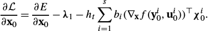
λ1ℓ=λ1ℓ+1+hts∑i=1bi(∇ϕf13)⊤χ1,iℓ,
χ1,iℓ=λ1ℓ+1+hts∑j=1bjajibi(∇ϕf13)⊤χ1,jℓ,

λ2ℓ=λ2ℓ+1+hts∑i=1bi(∇mℓf13∇mℓf23)⊤(χ1,iℓχ2,iℓ),

χ2,iℓ=λ2ℓ+1+hts∑j=1bjajibi(∇mℓf13∇mℓf23)⊤(χ1,jℓχ2,jℓ).

The final states of the adjoints λ1![]() and λ2
and λ2![]() are given by the partial derivatives with respect to the final states ϕN−1
are given by the partial derivatives with respect to the final states ϕN−1![]() and mN−1
and mN−1![]() , respectively:
, respectively:
λ1N−1=−∇PϕN−1E3(m,ϕ)=−∇ASimh(˜I0,I1)∇h˜I0,
λ2N−1=−∇mN−1E3(m,ϕ)=0.
The update of the initial momentum m0![]() , which is the initial value influencing the complete model via Eqs. (13.54)–(13.56) is given by adapting (13.41):
, which is the initial value influencing the complete model via Eqs. (13.54)–(13.56) is given by adapting (13.41):
∂L∂m0=∂E3(m,ϕ)∂m0−λ20=hvKm0−λ20.
13.6 Discretization in multiple dimensions
This section generalizes the equations from Section 13.4 and Section 13.5 to multidimensional LDDMM registration problems. Multidimensional formulations can easily be obtained from the one-dimensional representation by defining appropriate discrete operators. We illustrate this here for the three-dimensional case, but the approach is adaptable to arbitrary dimensions. For the computation of distance measures and their derivatives, we refer to [66, p. 95].
13.6.1 Discretization of the regularizer
The number of image voxels per dimension is denoted as Mi![]() , i=1,…,3
, i=1,…,3![]() , and the number of nodal grid points as ni
, and the number of nodal grid points as ni![]() . We define the total number of voxels and grid points as
. We define the total number of voxels and grid points as
M≔3∏i=1Mi,n≔3∏i=1ni.

The discrete images are thus I0,I1∈RM![]() , and the velocities are discretized as v∈R3n×N
, and the velocities are discretized as v∈R3n×N![]() . Our domain has a box shape: ˉΩ=[ω1,ω2]×[ω3,ω4]×[ω5,ω6]⊂R3
. Our domain has a box shape: ˉΩ=[ω1,ω2]×[ω3,ω4]×[ω5,ω6]⊂R3![]() . The resulting cell widths are hI1=ω2−ω1M1
. The resulting cell widths are hI1=ω2−ω1M1![]() , hI2=ω4−ω3M2
, hI2=ω4−ω3M2![]() , hI3=ω6−ω5M3
, hI3=ω6−ω5M3![]() for the images and hv1=ω2−ω1n1−1
for the images and hv1=ω2−ω1n1−1![]() , hv2=ω4−ω3n2−1
, hv2=ω4−ω3n2−1![]() , hv3=ω6−ω5n3−1
, hv3=ω6−ω5n3−1![]() for the velocities and transformations. For the computation of the regularizer, we need the volume of one cell that is defined as
for the velocities and transformations. For the computation of the regularizer, we need the volume of one cell that is defined as
hv≔hv1hv2hv3.
The construction for the discrete Laplacian is achieved using Kronecker products (see [66, p. 122]):
Δ=Idn3⊗Idn2⊗Δhv1+Idn3⊗Δhv2⊗Idn1+Δhv3⊗Idn2⊗Idn1,
where Δhiv![]() is the finite difference matrix given in (13.24), which is used to compute the second derivative in the ith dimension of one component of the velocities v. Hence we can write the multidimensional regularization matrix as an extension of (13.23):
is the finite difference matrix given in (13.24), which is used to compute the second derivative in the ith dimension of one component of the velocities v. Hence we can write the multidimensional regularization matrix as an extension of (13.23):
L=(γIdn−αΔ)β∈Rn×n.
This makes multiplication of L with one component of the vector-valued velocities at each discretization time point possible. As in Regh![]() , the velocities are integrated over time after multiplication with the Helmholtz operator, and L has to be multiplied with all components and for all times. We use copies of L for a short description but do not keep the copies in memory. In fact, as L is sparse, we implemented the multiplication with L without building the matrix. The corresponding matrix ˉL
, the velocities are integrated over time after multiplication with the Helmholtz operator, and L has to be multiplied with all components and for all times. We use copies of L for a short description but do not keep the copies in memory. In fact, as L is sparse, we implemented the multiplication with L without building the matrix. The corresponding matrix ˉL![]() is
is
ˉL≔Id3N⊗L,
and the matrix for the proper weighting of cells between grid points that are located at the boundaries of the box is realized as in (13.25), yielding
W≔WN⊗Id3⊗Wn3⊗Wn2⊗Wn1.
The discrete regularization energy is then given by applying the trapezoidal rule:
Regh(ˉv)≔hvht2ˉv⊤ˉL⊤WˉLˉv.
The vector ˉv∈R3nN![]() is the linearized matrix v, that is, the velocities are stacked up dimension-by-dimension for one time tℓ
is the linearized matrix v, that is, the velocities are stacked up dimension-by-dimension for one time tℓ![]() : First, all x-components of the velocities (v1ℓ∈Rn
: First, all x-components of the velocities (v1ℓ∈Rn![]() ), then all y-components (v2ℓ∈Rn
), then all y-components (v2ℓ∈Rn![]() ), and finally all z-components (v3ℓ∈Rn
), and finally all z-components (v3ℓ∈Rn![]() ) are stored. Then the same is done with the next time point, and so on. In the following equation we summarize this procedure using subvectors viℓ
) are stored. Then the same is done with the next time point, and so on. In the following equation we summarize this procedure using subvectors viℓ![]() , i=1
, i=1![]() , 2, 3, ℓ=0,1,…,N−1
, 2, 3, ℓ=0,1,…,N−1![]() , of v:
, of v:
v≔(v10v11…v1N−1v20v21…v2N−1v30v31…v3N−1).
For the shooting model, the kernel K is needed. As in the one-dimensional case, it is defined as
K=(L⊤L)−1∈Rn×n.
Note that the matrix K is not stored, but equation systems are solved to obtain the momentum fields from the velocity fields; see Section 13.5.5.
13.6.2 Integrands and associated gradients for the Runge–Kutta methods
To solve the Runge–Kutta integration (13.34) and in particular the adjoint equations (13.39), the specifications of the right-hand side function f and its derivatives are required. We distinguish here solutions of the transport equation (for a relaxation approach) and direct solutions of the LDDMM optimality conditions (for shooting). In the first case we consider image-based and map-based solutions. As the map-based solution has the advantage that considerably less image artifacts occur during numerical solution of the transport equation (see also Section 13.8.1), we will focus on this adaption for the shooting approach. Additionally, the shooting approach eliminates the dependency on the velocity v as it can be computed from the state variables. To evaluate f and solve the adjoint equations, we will need matrices to numerically compute the first derivative. In three dimensions these matrices are [66, p. 122]:
ˉD□1≔Id∘3⊗Id∘2⊗D□1,
ˉD□2≔Id∘3⊗D□2⊗Id∘1,
ˉD□3≔D□3⊗Id∘2⊗Id∘1,
where the subscripts denote the directions of the partial derivatives (x, y, and z), and (□,∘)∈{(I,M),(v,n)}![]() .
.
13.6.2.1 IBR model
We start with the discretization of the relaxation approach with transportation of images, that is, model (13.10). This is the simplest case as the state X corresponds to the vectorized images I=(Iℓ)N−1ℓ=0∈RM×N![]() only. The control variables are the discretized velocities v∈R3n×N
only. The control variables are the discretized velocities v∈R3n×N![]() . We want to transport the images with all their details and bring the velocities to the image resolution using the trilinear interpolation matrix P∈RM×n
. We want to transport the images with all their details and bring the velocities to the image resolution using the trilinear interpolation matrix P∈RM×n![]() ; see Section 13.4.1 and references therein. With the notation Pviℓ=:ˆviℓ
; see Section 13.4.1 and references therein. With the notation Pviℓ=:ˆviℓ![]() , i=1
, i=1![]() , 2, 3, ℓ=0,…,N−1
, 2, 3, ℓ=0,…,N−1![]() , the discretized transport equation becomes
, the discretized transport equation becomes
f1(Iℓ,vℓ)=−3∑i=1diag(ˉDIiIℓ)ˆviℓ.

The corresponding derivatives are:
∇Iℓf1(Iℓ,vℓ)=−3∑i=1diag(ˆviℓ)ˉDIi,
∇vℓf1(Iℓ,vℓ)=−diag((ˉDI1+ˉDI2+ˉDI3)Iℓ)P.
For the adjoint system, we need the final state of λ∈RM×N![]() , which is already given in (13.47) but is repeated here for completeness:
, which is already given in (13.47) but is repeated here for completeness:
λN−1=−∇ASimh(IN−1,I1).
As our objective function is essentially the same as for the one-dimensional case given in (13.45), combining (13.46) and (13.78) yields for the derivative of the regularizer with respect to the velocities:
∇vE1(IN−1,v)=hvhtˉLWˉLˉv.
13.6.2.2 MBR model
In the map-based case we transport all the coordinates (ϕ1![]() , ϕ2
, ϕ2![]() , ϕ3
, ϕ3![]() ) individually, that is, we have as many transport equations as there are spatial dimensions. The discrete transformation maps are ordered as
) individually, that is, we have as many transport equations as there are spatial dimensions. The discrete transformation maps are ordered as
ϕ≔(ϕ10ϕ11…ϕ1N−1ϕ20ϕ21…ϕ2N−1ϕ30ϕ31…ϕ3N−1)∈R3n×N.

Thus ϕ and v have the same discretization, and the transport equations do not need any further interpolations and hence no matrix/operator P:
f2(ϕℓ,vℓ)=−(∑3i=1diag(ˉDviϕ1ℓ)viℓ∑3i=1diag(ˉDviϕ2ℓ)viℓ∑3i=1diag(ˉDviϕ3ℓ)viℓ).
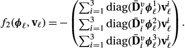
The gradients with respect to the state variable ϕ for the individual components of (13.90) can be expressed by the Kronecker delta as the transport in the different spatial directions is decoupled:
∇ϕlℓfj2(ϕℓ,vℓ)=−δj,l3∑i=1diag(viℓ)ˉDvi,j,l=1,2,3.

The derivatives with respect to the control variable v are
∇vℓf2(ϕℓ,vℓ)=−(diag(ˉDvjϕiℓ))3i,j=1.
To complete our adjoint system, we also need the final state of the adjoint variables λN−1![]() . Again, we abbreviate the transformed template images as ˜I0=I0∘(ˉPϕN−1)
. Again, we abbreviate the transformed template images as ˜I0=I0∘(ˉPϕN−1)![]() , and ∘ denotes trilinear interpolation on the grid ˉPϕN−1
, and ∘ denotes trilinear interpolation on the grid ˉPϕN−1![]() . Here the matrix ˉP
. Here the matrix ˉP![]() contains three copies of P and converts each dimension of ϕN−1
contains three copies of P and converts each dimension of ϕN−1![]() to cell-centered points:
to cell-centered points:
ˉP=(PPP)∈R3ˉm×3n.

The final state is similar to the one-dimensional case given in (13.50), but each transformation component is treated individually:
λN−1=−diag(∇h˜I0)(∇ASimh(˜I0,I1)∇ASimh(˜I0,I1)∇ASimh(˜I0,I1)).
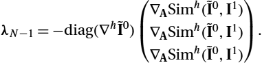
Here ∇h˜I0∈R3M![]() is the discrete gradient of the image ˜I0∈RM
is the discrete gradient of the image ˜I0∈RM![]() , where the first M components are the partial derivatives in the x-direction, then the y- and finally the z-directions follow. The arguments given at the end of Section 13.5.4 still apply, and the adjoint equations are solved on the image resolution using the matrix P appropriately and storing the adjoint only when necessary at high resolution. As the regularization energy is the same as in the image-based model:
, where the first M components are the partial derivatives in the x-direction, then the y- and finally the z-directions follow. The arguments given at the end of Section 13.5.4 still apply, and the adjoint equations are solved on the image resolution using the matrix P appropriately and storing the adjoint only when necessary at high resolution. As the regularization energy is the same as in the image-based model:
E2(ϕN−1,v)=Regh(ˉv)+Simh(˜I0,I1).
The derivative with respect to the velocities is also the same:
∇vE2(ϕN−1,v)=hvhtˉLWˉLˉv.
13.6.2.3 MBS model
Instead of solving map-based equations to decouple spatial transformations from the objects to be transported, we can directly solve the EPDiff equation (13.55) with the constraint (13.56) to optimize the discrete energy
E3(m,ϕ)=hv23∑i=1(mi0)⊤Kmi0+Simh(˜I0,I1).
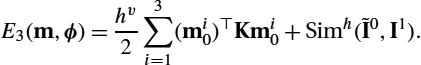
To compute the transformed source image, we still need the transformation ϕ and thus (13.90) to compute its evolution. The resulting discrete right-hand side function has six components:
fj3(ϕℓ,mℓ)=−3∑i=1diag(ˉDviϕjℓ)Kmiℓ,
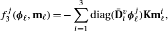
fj+33(mℓ)=−3∑i=1(diag(ˉDvimjℓ)Kmiℓ+diag(ˉDvjKmiℓ)miℓ+diag(mjℓ)ˉDviKmiℓ)
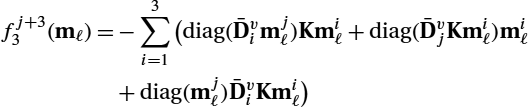
for j=1,2,3![]() , where we used viℓ=Kmiℓ
, where we used viℓ=Kmiℓ![]() , i=1,2,3
, i=1,2,3![]() and ℓ=0,…,N−1
and ℓ=0,…,N−1![]() . A useful relation when computing the derivatives of the right-hand side function is
. A useful relation when computing the derivatives of the right-hand side function is
∇mlℓvjℓ=δj,lK={0,l≠j,K,l=j.

The resulting derivatives of f3![]() are
are
∇ϕlℓfj3=−δj,l3∑i=1diag(Kmiℓ)ˉDvi,

∇mlℓfj3=−diag(ˉDvlϕjℓ)K,
∇ϕlℓfj+33=0,
∇mlℓfj+33=−(diag(ˉDvlmjℓ)+diag(mlℓ)ˉDvj+diag(mjℓ)ˉDvl)K−diag(ˉDvjKmlℓ)−δj,l3∑i=1(diag(ˉDviKmiℓ)+diag(Kmiℓ)ˉDvi),

for j, l=1,2,3![]() .
.
As we have six state variables ϕ1ℓ![]() , ϕ2ℓ
, ϕ2ℓ![]() , ϕ3ℓ
, ϕ3ℓ![]() and m1ℓ
and m1ℓ![]() , m2ℓ
, m2ℓ![]() , m3ℓ
, m3ℓ![]() that are updated using Runge–Kutta methods with the right-hand sides f13,…,f63
that are updated using Runge–Kutta methods with the right-hand sides f13,…,f63![]() , there are also six adjoint variables λ1ℓ,…,λ6ℓ
, there are also six adjoint variables λ1ℓ,…,λ6ℓ![]() with intermediate variables χ1,iℓ,…,χ6,iℓ
with intermediate variables χ1,iℓ,…,χ6,iℓ![]() for i=1,…,s
for i=1,…,s![]() and ℓ=0,…,N−1
and ℓ=0,…,N−1![]() . The derivatives of f3
. The derivatives of f3![]() , given in (13.101)–(13.104), are used in the adjoint Runge–Kutta system (13.39) to update the adjoint variables. It remains to give a complete description are the final states of the adjoints λ1N−1,…,λ6N−1
, given in (13.101)–(13.104), are used in the adjoint Runge–Kutta system (13.39) to update the adjoint variables. It remains to give a complete description are the final states of the adjoints λ1N−1,…,λ6N−1![]() . They are given by the partial derivatives of E3
. They are given by the partial derivatives of E3![]() with respect to the final states ϕN−1
with respect to the final states ϕN−1![]() and mN−1
and mN−1![]() , respectively. The first three equations are the same as in (13.94), but we repeat them for completeness, the last λ4N−1
, respectively. The first three equations are the same as in (13.94), but we repeat them for completeness, the last λ4N−1![]() , λ5N−1
, λ5N−1![]() , λ6N−1
, λ6N−1![]() vanish as the energy depends on the initial momentum and not on the final one:
vanish as the energy depends on the initial momentum and not on the final one:
(λ1N−1λ2N−1λ3N−1)=−diag(∇h˜I0)(∇ASimh(˜I0,I1)∇ASimh(˜I0,I1)∇ASimh(˜I0,I1)),
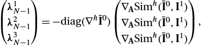
λjN−1=0,j=4,5,6.
The update of the initial momentum m0![]() that is the initial value influencing the complete model via Eqs. (13.98) and (13.99) is given by adapting (13.41):
that is the initial value influencing the complete model via Eqs. (13.98) and (13.99) is given by adapting (13.41):
∂L∂m0=∂E3(m,ϕ)∂m0−(λ40,λ50,λ60)⊤=(hvKm10−λ40hvKm20−λ50hvKm30−λ60).
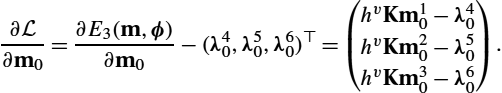
13.7 Multilevel registration and numerical optimization
A key concept of most image registration algorithms is the registration on multiple levels. By computing solutions to registration problems with images whose resolution is gradually increased the risk of getting stuck in a local minimum is reduced [66, p. 13]. Additionally, the numerical optimization on the coarse levels with images consisting of fewer pixels/voxels is faster but gives a good approximation for the solution on the next level, further reducing runtime.
Because of these two reasons, we also employed a multilevel registration. The number of points in space varied during the multilevel optimization such that the grid spacing was halved on each finer level. After choosing n1j,j=1,2,3![]() , the number of grid points is hence given as nij≔(n1j−1)2i−1+1
, the number of grid points is hence given as nij≔(n1j−1)2i−1+1![]() . Given images I0,I1∈RM1×M2×M3
. Given images I0,I1∈RM1×M2×M3![]() , smoothed and downsampled versions I0i,I1i∈RMi1×Mi2×Mi3
, smoothed and downsampled versions I0i,I1i∈RMi1×Mi2×Mi3![]() with Mij=⌊Mj⋅2−F+i⌋
with Mij=⌊Mj⋅2−F+i⌋![]() were computed for j=1,2,3
were computed for j=1,2,3![]() and i=1,…,F
and i=1,…,F![]() [66, p. 40]. Problems (13.10), (13.14), and (13.17) were then solved using a coarse-to-fine resolution multilevel strategy with
[66, p. 40]. Problems (13.10), (13.14), and (13.17) were then solved using a coarse-to-fine resolution multilevel strategy with ![]() levels. For the (bi/tri)linear interpolation, which is needed to compute the transformed source image
levels. For the (bi/tri)linear interpolation, which is needed to compute the transformed source image ![]() , we used the Matlab code provided by [66].
, we used the Matlab code provided by [66].
The discretization resolution of the velocities, momenta, and transformations can be chosen by the user. One drawback is that (for the 3D lung registration, we are tackling) choosing ![]() exceeds common memory limitations and results in an extremely expensive solution of the constraint (13.34) and adjoint Eqs. (13.39). As motivated before, by LDDMM design v and ϕ are assumed to be smooth functions, and it is usually not necessary to use a high resolution for v and ϕ. This motivates our choice of
exceeds common memory limitations and results in an extremely expensive solution of the constraint (13.34) and adjoint Eqs. (13.39). As motivated before, by LDDMM design v and ϕ are assumed to be smooth functions, and it is usually not necessary to use a high resolution for v and ϕ. This motivates our choice of ![]() .
.
To maintain accurate registrations, we use all given image information (at the highest resolution) by solving the adjoint equations at image resolution as given in the final adjoint state Eqs. (13.87), (13.94), and (13.105) for the different approaches, respectively. Empirically, ![]() worked well for lung CT registrations in our previous work [76]. The appropriate (trilinear) interpolations for the change between grids were realized with P. As mentioned before, P is sparse but large, but P does not need to be kept in memory [51,80]. We use matrix notation but implemented a matrix-free operator following [51,80].
worked well for lung CT registrations in our previous work [76]. The appropriate (trilinear) interpolations for the change between grids were realized with P. As mentioned before, P is sparse but large, but P does not need to be kept in memory [51,80]. We use matrix notation but implemented a matrix-free operator following [51,80].
It is useful to start a registration with the result of a preregistration ![]() . Given a (preferably diffeomorphic) transformation ψ only the initial conditions of the problems (13.10), (13.14), and (13.17) have to be adapted:
. Given a (preferably diffeomorphic) transformation ψ only the initial conditions of the problems (13.10), (13.14), and (13.17) have to be adapted: ![]() or
or ![]() , respectively. In discrete notation these equations read
, respectively. In discrete notation these equations read ![]() and
and ![]() .
.
The number of simulated points in time N is very important for the LDDMM registration. From the stability function [41, p. 16] for the explicit Runge–Kutta 4th-order the maximal admissible time step for solving the discrete transport equation can be derived as [73, p. 175]
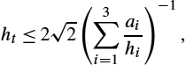
where ![]() is the expected maximal magnitude of movement in direction
is the expected maximal magnitude of movement in direction ![]() . An intermediate temporal step size was determined as
. An intermediate temporal step size was determined as

Using 2.8 instead of ![]() adds a safety margin shielding against inaccuracies due to discretization errors. Additionally, as we are interested in integer values N, we compute:
adds a safety margin shielding against inaccuracies due to discretization errors. Additionally, as we are interested in integer values N, we compute:
which results in an even larger safety margin. According to (13.108), the time step has to decrease when the grid step size decreases, and therefore we determine ![]() at the finest level (
at the finest level (![]() ). The main difficulty left is the estimation of the maximal motion that occurred to obtain
). The main difficulty left is the estimation of the maximal motion that occurred to obtain ![]() ,
, ![]() . However, for typical medical registration scenarios in which we are interested, upper bounds for the motion that should be recovered by the registration are available. In the case of lung CT registration, even from full inspiration to full expiration, the maximal amplitude can be estimated (with a large safety margin) as 100 mm; see [17] for example datasets.
. However, for typical medical registration scenarios in which we are interested, upper bounds for the motion that should be recovered by the registration are available. In the case of lung CT registration, even from full inspiration to full expiration, the maximal amplitude can be estimated (with a large safety margin) as 100 mm; see [17] for example datasets.
The discretized objective functions (13.45), (13.95), and (13.97) were optimized with an L-BFGS approach [71, p. 176] saving the last 5 iteration vectors for approximation of the inverse Hessian. The maximum number of iterations was set to ![]() . Additional stopping criteria proposed in [66, p. 78] were used to terminate the optimization on each level. During the optimization, an Armijo line search with parameters
. Additional stopping criteria proposed in [66, p. 78] were used to terminate the optimization on each level. During the optimization, an Armijo line search with parameters ![]() ,
, ![]() , and
, and ![]() was used to guarantee a decrease of the objective function [71, p. 33]. The gradients used for the optimization are given in the last equation of (13.39) for the relaxation approaches and in (13.107) for the shooting approach. They are detailed for IBR in Section 13.6.2.1, Section 13.6.2.2, and Section 13.6.2.3 for the IBR, MBR, and MBS models, respectively. Before using the gradients of the relaxation methods for optimization, they are smoothed to obtain the Hilbert gradients (13.9) by N-fold application of K. As
was used to guarantee a decrease of the objective function [71, p. 33]. The gradients used for the optimization are given in the last equation of (13.39) for the relaxation approaches and in (13.107) for the shooting approach. They are detailed for IBR in Section 13.6.2.1, Section 13.6.2.2, and Section 13.6.2.3 for the IBR, MBR, and MBS models, respectively. Before using the gradients of the relaxation methods for optimization, they are smoothed to obtain the Hilbert gradients (13.9) by N-fold application of K. As ![]() coincides with the second order derivative of
coincides with the second order derivative of ![]() , this can be viewed as a Newton step only with respect to the regularization term.
, this can be viewed as a Newton step only with respect to the regularization term.
The determinant of the Jacobian of the transformation can be used to find singularities (foldings of the grid or grid cells with vanishing volume) or to evaluate whether local volume expansion or contraction occurs. Therefore it is a good criterion to check for local invertibility [24, p. 222] and to find out if the computed transformation is a diffeomorphism. We computed Jacobian determinant values ![]() ,
, ![]() on the last registration level F with the dedicated method used for hyperelastic regularization [13] in the FAIR [66] Matlab toolbox.5 The computed transformation
on the last registration level F with the dedicated method used for hyperelastic regularization [13] in the FAIR [66] Matlab toolbox.5 The computed transformation ![]() contained sporadically negative Jacobians for some parameter choices (and thus was not diffeomorphic), which resulted from inaccuracies that occur when solving the transport equation for iterated time steps with the fourth-order Runge–Kutta method. Therefore, we used the obtained velocities v to compute the final transformation
contained sporadically negative Jacobians for some parameter choices (and thus was not diffeomorphic), which resulted from inaccuracies that occur when solving the transport equation for iterated time steps with the fourth-order Runge–Kutta method. Therefore, we used the obtained velocities v to compute the final transformation ![]() in a slightly different manner. The fourth-order Runge–Kutta method (13.34) with the right-hand side given in (13.90) was solved for one time step starting from the identity grid
in a slightly different manner. The fourth-order Runge–Kutta method (13.34) with the right-hand side given in (13.90) was solved for one time step starting from the identity grid ![]() with varying velocities
with varying velocities ![]() for
for ![]() to obtain small deformations
to obtain small deformations ![]() . These steps were then concatenated (starting from the preregistration ψ) using trilinear interpolation to obtain the total transformation
. These steps were then concatenated (starting from the preregistration ψ) using trilinear interpolation to obtain the total transformation
If each of the transformations ψ, ![]() for
for ![]() is diffeomorphic, then also φ is diffeomorphic [69,50,104]. However, repeated interpolations are time-consuming and difficult to handle when solving the adjoint system consistently. Therefore, during the numerical optimization, the methods presented in Section 13.5 and Section 13.6 are used to estimate the discrete velocity fields v. After the optimization is finished, the final transformation φ is computed within a postprocessing step according to (13.111) to achieve a transformation that is guaranteed to be diffeomorphic.
is diffeomorphic, then also φ is diffeomorphic [69,50,104]. However, repeated interpolations are time-consuming and difficult to handle when solving the adjoint system consistently. Therefore, during the numerical optimization, the methods presented in Section 13.5 and Section 13.6 are used to estimate the discrete velocity fields v. After the optimization is finished, the final transformation φ is computed within a postprocessing step according to (13.111) to achieve a transformation that is guaranteed to be diffeomorphic.
13.8 Experiments and results
This section shows experimental results on 2D radiographs of hands (Section 13.8.1) and 3D CT lung images (Section 13.8.2).
13.8.1 2D registration of hand radiographs
We illustrate our approach on a 2D dataset. The dataset consists of two ![]() pixel radiographs of human right hands of two different patients (see Fig. 13.3(A) and Fig. 13.3(F)). The dataset has previously been used in [65] and is part of the FAIR Matlab toolbox [66]. Before applying the LDDMM methods, the images were affinely preregistered using FAIR with SSD distance measure on the coarsest level of the image pyramid. SSD was also used for the LDDMM methods. According to (13.23),
pixel radiographs of human right hands of two different patients (see Fig. 13.3(A) and Fig. 13.3(F)). The dataset has previously been used in [65] and is part of the FAIR Matlab toolbox [66]. Before applying the LDDMM methods, the images were affinely preregistered using FAIR with SSD distance measure on the coarsest level of the image pyramid. SSD was also used for the LDDMM methods. According to (13.23), ![]() regularity with
regularity with ![]() is necessary for
is necessary for ![]() (and thus
(and thus ![]() ) to guarantee diffeomorphic solutions. However,
) to guarantee diffeomorphic solutions. However, ![]() is the limit case, and we therefore decided to employ
is the limit case, and we therefore decided to employ ![]() . The other parameters were determined empirically and fixed for all three approaches to
. The other parameters were determined empirically and fixed for all three approaches to ![]() ,
, ![]() ,
, ![]() ,
, ![]() and
and ![]() ,
, ![]() ,
, ![]() . The second column of Fig. 13.3 shows the results of the preregistration. The following columns display the results of the IBR, MBR, and MBS approaches. Properties of the computed transformation maps are most obvious in the Jacobian determinant visualizations in the second row of Fig. 13.3. The shooting approach clearly produces smoother transformations than both relaxation approaches. Furthermore, the volume change for the relaxation approaches is locally quite different indicating that advecting the non-smooth images (via the transport equation) introduces more numerical problems than advecting the comparatively smooth spatial transformations. The resulting distortion in the deformed moving image is apparent when comparing Fig. 13.3(C) and Fig. 13.3(D). In the former oscillations next to sharp edges in the images arise, whereas the latter image has the same quality as the undeformed moving image.
. The second column of Fig. 13.3 shows the results of the preregistration. The following columns display the results of the IBR, MBR, and MBS approaches. Properties of the computed transformation maps are most obvious in the Jacobian determinant visualizations in the second row of Fig. 13.3. The shooting approach clearly produces smoother transformations than both relaxation approaches. Furthermore, the volume change for the relaxation approaches is locally quite different indicating that advecting the non-smooth images (via the transport equation) introduces more numerical problems than advecting the comparatively smooth spatial transformations. The resulting distortion in the deformed moving image is apparent when comparing Fig. 13.3(C) and Fig. 13.3(D). In the former oscillations next to sharp edges in the images arise, whereas the latter image has the same quality as the undeformed moving image.
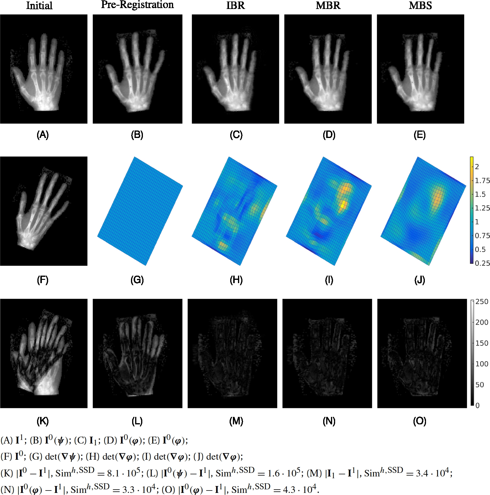
 ,
,  , N = 10.
Due to their representational flexibility, the relaxation approaches reach a slightly better image match as visible in the last row in the difference images. In particular the ring and the baby finger of the shooting result lack some width compared to the fixed image and are closer to the width of the fingers in the undeformed source image ![]() . The inferior image match is quantified by the three SSD values for the different approaches. These values also indicate that due to the image deterioration induced by the IBR approach, the image match is not as good as with the MBR approach. However, although the differences in image mismatch when comparing IBR and MBR to MBS are relatively small, the difference in transformation field smoothness is remarkable.
. The inferior image match is quantified by the three SSD values for the different approaches. These values also indicate that due to the image deterioration induced by the IBR approach, the image match is not as good as with the MBR approach. However, although the differences in image mismatch when comparing IBR and MBR to MBS are relatively small, the difference in transformation field smoothness is remarkable.
13.8.2 3D registration of lung CT data
To demonstrate the suitability of our method for 3D lung CT data, we make use of the publicly available DIR-Lab datasets [16,17,15]. These datasets were acquired from 20 subjects (with or without pulmonary diseases) during the inhale and exhale phases and are either part of the COPDgene study [77] or 3D volumes from 4DCT scans. The number of voxels per axial slice is ![]() for all COPD datasets [17] and 4DCT datasets 6 to 10 [16]. For 4DCT datasets 1 to 5 [15], the number of voxels per axial slice is
for all COPD datasets [17] and 4DCT datasets 6 to 10 [16]. For 4DCT datasets 1 to 5 [15], the number of voxels per axial slice is ![]() . Each slice has a thickness of 2.5 mm, and the number of slices ranges between 94 and 135. The axial resolution varies from
. Each slice has a thickness of 2.5 mm, and the number of slices ranges between 94 and 135. The axial resolution varies from ![]() to
to ![]() for the COPD data [17], is
for the COPD data [17], is ![]() for 4DCT datasets 6 to 10 [16] and ranges from
for 4DCT datasets 6 to 10 [16] and ranges from ![]() to
to ![]() for 4DCT datasets 1 to 5 [15]. Additionally to the images, 300 expert-placed landmarks per image are provided. These landmarks can be used for evaluation of registration accuracy.
for 4DCT datasets 1 to 5 [15]. Additionally to the images, 300 expert-placed landmarks per image are provided. These landmarks can be used for evaluation of registration accuracy.
Statistics of the Jacobian of the computed deformation fields are often used to evaluate the plausibility of the registration see, for example, [68] for the application to lung CT registration. Therefore we evaluate the Jacobians for the computed final transformation φ to estimate the reconstructed volume change of local regions of the lung and to assess for unreasonable expansions, contractions, or foldings of lung tissue.
In many clinical applications only information within the lungs is required, for example, for the staging and phenotyping of COPD [32]. Although the motion of the lung induced by respiration is smooth (making LDDMM a suitable registration model), motion discontinuities occur at the interface with the ribcage [88]. These discontinuities interfere with the LDDMM model, although in [78] a modification is presented, which applies special kernels to allow for discontinuous motions. However, as we are only interested in the alignment of the lungs, we generated lung segmentations using the method proposed in [53] and masked the CT scans to remove unnecessary image information. Hence an adaptation of our models is no longer necessary. In addition to the masking the images were cropped such that in each direction approximately 5 mm of margin were retained. For all registrations, the inhale scans were used as target images and the exhale scans as source images.
In the following experiments we used a thin-plate spline (TPS) preregistration. The TPS is based on keypoints acquired with the method in [46], which were also used for the registration of difficult COPD data with remarkably accurate results [82]. However, the TPS preregistration with these keypoints may produce transformations with foldings (i.e., negative Jacobians). Therefore, to ensure that ψ is diffeomorphic, we removed keypoints whose set of six nearest neighbors changes after TPS computation by more than one point, suggesting a violation of topology preservation. This procedure reduced the number of keypoints to approximately one quarter of the original number and results in decreased accuracy of the preregistration; see Table 13.2. The subsequent registration with our LDDMM methods MBR and MBS retained the diffeomorphic property of the estimated transformation, which might not be the case for small deformation methods; see the discussion in [23].
Table 13.2
Mean landmark distances of the 300 landmark pairs after registration with state-of-the-art methods. All values are given in mm and were computed after rounding to the next voxel center.
| blank cell | Mean landmark distance after registration in mm | ||||||||
|---|---|---|---|---|---|---|---|---|---|
| Case | Initial | MILO | MRF | LMP | DIS-CO | isoPTV | Prereg. | MBR | MBS |
| [18] | [46] | [74] | [82] | [99] | |||||
| 4DCT1 | 3.89 | 0.74 | 0.76 | 0.80 | 0.74 | 0.76 | |||
| 4DCT2 | 4.34 | 0.78 | 0.77 | 0.75 | 0.80 | 0.82 | |||
| 4DCT3 | 6.94 | 0.91 | 0.90 | 0.95 | 0.93 | 0.95 | |||
| 4DCT4 | 9.83 | 1.24 | 1.24 | 1.39 | 1.24 | 1.31 | |||
| 4DCT5 | 7.48 | 1.17 | 1.12 | 1.25 | 1.10 | 1.11 | |||
| 4DCT6 | 10.89 | 0.90 | 0.85 | 1.04 | 0.86 | 0.87 | |||
| 4DCT7 | 11.03 | 0.87 | 0.80 | 1.09 | 0.83 | 0.88 | |||
| 4DCT8 | 14.99 | 1.04 | 1.34 | 1.20 | 1.11 | 1.10 | |||
| 4DCT9 | 7.92 | 0.98 | 0.92 | 1.10 | 0.96 | 0.93 | |||
| 4DCT10 | 7.30 | 0.89 | 0.82 | 1.09 | 0.88 | 0.90 | |||
| Average | 8.46 | 0.95 | 0.95 | 1.07 | 0.95 | 0.96 | |||
| COPD1 | 26.34 | 0.93 | 1.00 | 1.21 | 0.79 | 0.77 | 1.15 | 1.12 | 0.91 |
| COPD2 | 21.79 | 1.77 | 1.62 | 1.97 | 1.46 | 2.22 | 2.18 | 1.49 | 1.49 |
| COPD3 | 12.64 | 0.99 | 1.00 | 1.06 | 0.84 | 0.82 | 1.19 | 0.97 | 0.96 |
| COPD4 | 29.58 | 1.14 | 1.08 | 1.64 | 0.74 | 0.85 | 1.32 | 0.89 | 0.97 |
| COPD5 | 30.08 | 1.02 | 0.96 | 1.46 | 0.71 | 0.77 | 1.18 | 0.79 | 0.92 |
| COPD6 | 28.46 | 0.99 | 1.01 | 1.34 | 0.64 | 0.86 | 1.27 | 0.84 | 0.92 |
| COPD7 | 21.60 | 1.03 | 1.05 | 1.16 | 0.79 | 0.74 | 1.32 | 0.92 | 0.93 |
| COPD8 | 26.46 | 1.31 | 1.08 | 1.54 | 0.77 | 0.81 | 1.47 | 1.03 | 1.03 |
| COPD9 | 14.86 | 0.86 | 0.79 | 0.99 | 0.62 | 0.83 | 1.02 | 0.75 | 0.73 |
| COPD10 | 21.81 | 1.23 | 1.18 | 1.39 | 0.86 | 0.92 | 1.51 | 1.02 | 1.09 |
| Average | 23.36 | 1.13 | 1.08 | 1.38 | 0.82 | 0.96 | 1.36 | 0.98 | 1.00 |
| Total Average | 15.91 | 1.13 | 1.08 | 1.16 | 0.82 | 0.96 | 1.21 | 0.96 | 0.98 |
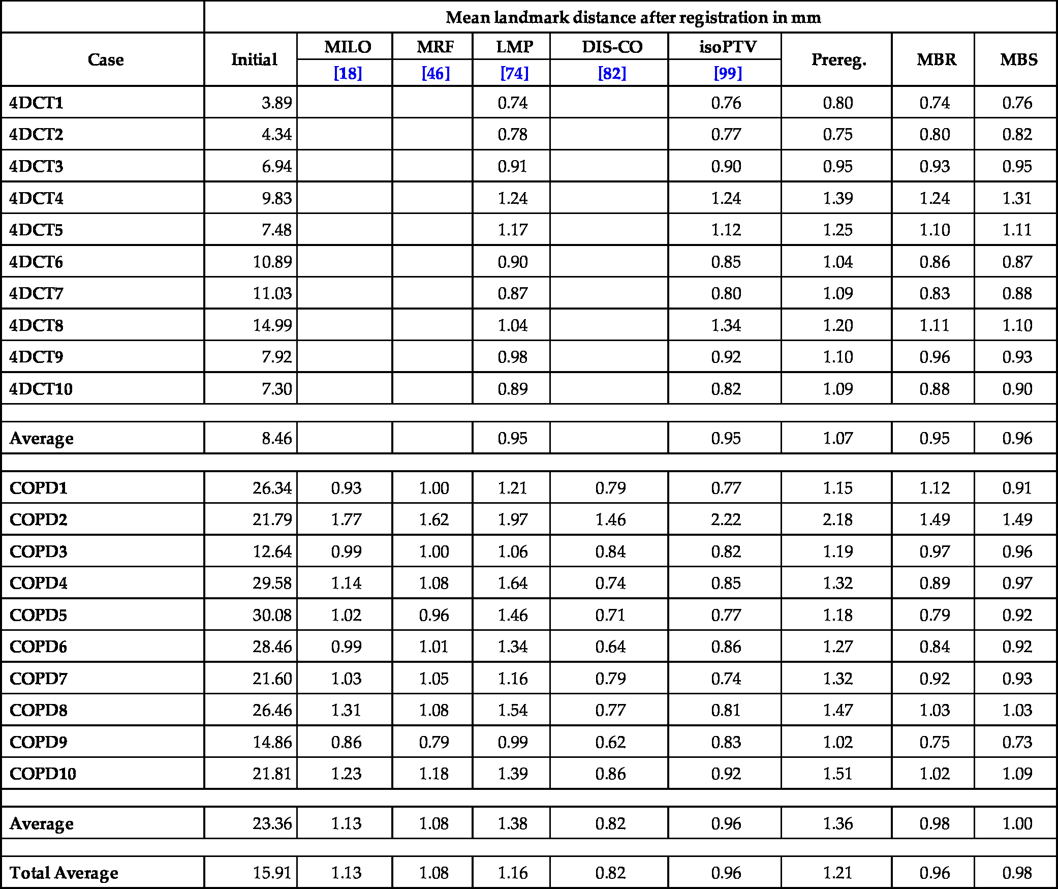
Due to the deteriorated quality of the deformed image of the IBR approach (see Section 13.8.1) and the interest in the volume change and plausibility of the transformation maps, we only applied the MBR and MBS approaches to the 3D lung datasets. We chose NGF as the distance measure, as it has been shown to work well on lung CT data; see Section 13.1. The same model parameters were used for all registrations: ![]() ,
, ![]() ,
, ![]() ,
, ![]() ,
, ![]() , and
, and ![]() . For the estimation of the time step
. For the estimation of the time step ![]() , we need an estimate for the maximal motion that may have occurred, which was denoted as
, we need an estimate for the maximal motion that may have occurred, which was denoted as ![]() ,
, ![]() , in Section 13.7. As the employed preregistration achieves a very good initial alignment and dramatically reduces the maximal motion required, we chose
, in Section 13.7. As the employed preregistration achieves a very good initial alignment and dramatically reduces the maximal motion required, we chose ![]() ,
, ![]() , and the number of time steps according to (13.110).
, and the number of time steps according to (13.110).
Registration results for dataset 4 of the COPD datasets are shown as coronal views in Fig. 13.4. The initial unaligned images are shown in the leftmost column; note the differences in noise level and volume for the exhale scan (![]() ) and the inhale scan (
) and the inhale scan (![]() ). The results for the preregistration ψ alone are very good and shown in the second column. Only smaller vessels and some lung boundaries show visually obvious mismatches. Our subsequent LDDMM registrations MBR and MBS, shown in the third and fourth columns, respectively, successfully handle these mismatches and produce visually very similar results. The second row shows that the Jacobian determinant maps for all registration approaches are smooth and positive. The largest volume changes occur near the mediastinum and might be influenced by the beating heart. Taking a closer look at the image of the Jacobian determinants of MBS (Fig. 13.4(H)) reveals that it is smoother than that of MBR (Fig. 13.4(G)) regarding variations in the left-right direction. Both approaches yield very smooth results in the anterior-superior direction. In particular, the lung volume decreases (Jacobian determinant values smaller than 1), which is what we expect during exhalation, which is modeled by our choice of using the inhale phase as the fixed image and the exhale phase as the moving image.
). The results for the preregistration ψ alone are very good and shown in the second column. Only smaller vessels and some lung boundaries show visually obvious mismatches. Our subsequent LDDMM registrations MBR and MBS, shown in the third and fourth columns, respectively, successfully handle these mismatches and produce visually very similar results. The second row shows that the Jacobian determinant maps for all registration approaches are smooth and positive. The largest volume changes occur near the mediastinum and might be influenced by the beating heart. Taking a closer look at the image of the Jacobian determinants of MBS (Fig. 13.4(H)) reveals that it is smoother than that of MBR (Fig. 13.4(G)) regarding variations in the left-right direction. Both approaches yield very smooth results in the anterior-superior direction. In particular, the lung volume decreases (Jacobian determinant values smaller than 1), which is what we expect during exhalation, which is modeled by our choice of using the inhale phase as the fixed image and the exhale phase as the moving image.
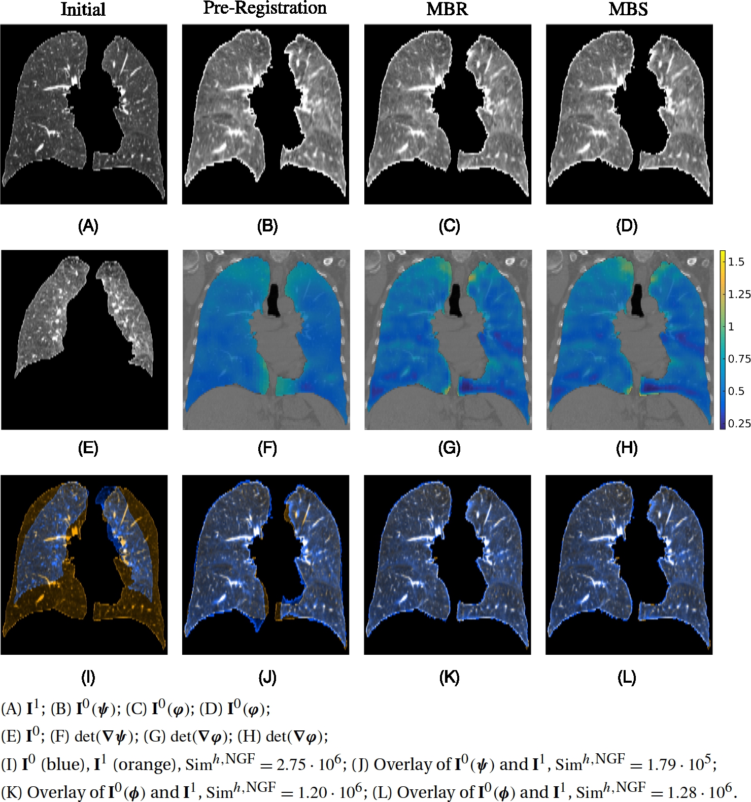
 ,
,  , N = 9.
Table 13.2 shows the mean landmark distances for all 20 datasets after MBR and MBS registration and allows for a comparison to reported results of state-of-the-art methods participating in the DIR-Lab benchmark.6 For the 4DCT data, all compared algorithms achieve similar results regarding landmark accuracy. Results on the DIR-Lab 4DCT data were not reported in the literature for MILO [18], MRF [46], and DIS-CO [82] and are therefore not listed. DIS-CO [82] achieves the best mean landmark distance (also called target registration error (TRE)) on the more challenging COPD data. The second best method regarding TRE is [99] but is closely followed by the MBR and the MBS approaches. The algorithm proposed in [99] does not use lung segmentations for image masking, but its total variation-based regularization allows for sliding motions. However, this also has the drawback that there is no guarantee that the estimated transformations contain no foldings.
The advantage of the MBR and MBS methods (ranking third and fourth regarding TRE) is that they produce transformation maps without foldings or implausible volume changes within the lungs; see Table 13.3. Only two other methods, LMP [74] and DIS-CO [82], can guarantee this regularity, and LMP achieves a worse TRE on the COPD data than both MBR and MBS.
Table 13.3
Minimum, mean, and standard deviation (SD) of the Jacobian determinant values of the computed transformations ![]() restricted to the lung volume. The mean value should be similar to the volume ratio (VR), which was computed as the ratio of exhale lung volume to inhale lung volume using the lung masks.
restricted to the lung volume. The mean value should be similar to the volume ratio (VR), which was computed as the ratio of exhale lung volume to inhale lung volume using the lung masks.
| MBR | MBS | ||||
|---|---|---|---|---|---|
| Case | VR | Min. | Mean ± SD | Min. | Mean±SD |
| 4DCT1 | 0.91 | 0.48 | 0.92±0.10 | 0.50 | 0.92±0.10 |
| 4DCT2 | 0.92 | 0.45 | 0.92±0.09 | 0.42 | 0.92±0.11 |
| 4DCT3 | 0.90 | 0.47 | 0.90±0.10 | 0.52 | 0.90±0.11 |
| 4DCT4 | 0.86 | 0.46 | 0.86±0.15 | 0.41 | 0.86±0.16 |
| 4DCT5 | 0.91 | 0.46 | 0.92±0.13 | 0.44 | 0.92±0.15 |
| 4DCT6 | 0.77 | 0.42 | 0.77±0.09 | 0.44 | 0.77±0.09 |
| 4DCT7 | 0.82 | 0.43 | 0.79±0.09 | 0.44 | 0.79±0.09 |
| 4DCT8 | 0.83 | 0.34 | 0.80±0.09 | 0.34 | 0.80±0.10 |
| 4DCT9 | 0.86 | 0.46 | 0.87±0.10 | 0.42 | 0.87±0.10 |
| 4DCT10 | 0.86 | 0.31 | 0.87±0.13 | 0.32 | 0.87±0.14 |
| COPD1 | 0.62 | 0.12 | 0.65±0.15 | 0.17 | 0.65±0.14 |
| COPD2 | 0.73 | 0.15 | 0.75±0.24 | 0.17 | 0.75±0.25 |
| COPD3 | 0.80 | 0.29 | 0.80±0.13 | 0.29 | 0.80±0.14 |
| COPD4 | 0.49 | 0.18 | 0.50±0.12 | 0.16 | 0.50±0.12 |
| COPD5 | 0.49 | 0.15 | 0.49±0.11 | 0.15 | 0.49±0.11 |
| COPD6 | 0.62 | 0.18 | 0.64±0.16 | 0.06 | 0.64±0.16 |
| COPD7 | 0.75 | 0.39 | 0.75±0.11 | 0.38 | 0.75±0.12 |
| COPD8 | 0.58 | 0.21 | 0.59±0.13 | 0.23 | 0.59±0.13 |
| COPD9 | 0.73 | 0.32 | 0.74±0.12 | 0.32 | 0.74±0.13 |
| COPD10 | 0.61 | 0.11 | 0.61±0.12 | 0.11 | 0.61±0.13 |

The Jacobians given in Table 13.3 show that the computed transformation field is indeed very smooth, as the standard deviation is small. Furthermore, the mean volume change is well correlated with the expected volume ratio, and no foldings of the grid occurred as the minimal Jacobian is always positive. To obtain diffeomorphic transformations φ from the previously computed ![]() in the discrete framework, we used the procedure described in Section 13.7. The transformations
in the discrete framework, we used the procedure described in Section 13.7. The transformations ![]() and φ show only small differences. The mean value of
and φ show only small differences. The mean value of ![]() computed over all 20 DIR-Lab datasets is 3.15 mm for the MBR method and 5.80 mm for the MBS method.
computed over all 20 DIR-Lab datasets is 3.15 mm for the MBR method and 5.80 mm for the MBS method.
All experiments were run on a PC with a single 3.4 GHz Intel i7-2600 quad-core CPU, 16 GB of RAM, and Ubuntu 14.04. Runtimes for the MBS approach ranged between 16 and 55 min with an average of 28 min. The peak memory consumption was 4.3 GB over all datasets. Analogously, for MBR, the runtimes ranged between 5 and 24 min with an average of 14 min and a peak memory consumption of 2.1 GB.
13.9 Discussion and conclusion
LDDMM is a popular registration method with nice mathematical properties that has successfully been applied to various applications; see, for example, [64] and references therein. The estimated deformation fields are guaranteed to be diffeomorphic, the deformation paths are geodesics, large displacements can be captured, and LDDMM induces a distance measure on images [7]. These properties, however, come with the drawbacks of a large computational burden, both with respect to runtime and memory consumption.
It is interesting that numerical approaches for LDDMM have not been explored in great depth, and the predominant solution approach is still optimize–discretize via gradient descent as proposed in [7]. Hence we chose to develop discretize–optimize schemes for relaxation and shooting, offering consistent numerical optimizations for the discretized energy, which, as discussed in [35], cannot be guaranteed for optimize–discretize approaches such as [7]. Formulating a discretized energy included the discretization of PDE constraints (mainly transport and scalar conservation equations), which we accomplished via an explicit fourth-order Runge–Kutta method as a good compromise between efficiency and accuracy. We also reduced memory consumption and runtime by representing velocities and transformation maps at lower spatial resolutions compared to the images. This is justified due to the smoothness of velocity fields and transformation maps and still allowed for high-quality registrations. Finally, our proposed methods can also be used with different image similarity measures, and we explored the use of NGF for lung registration.
We demonstrated the characteristics of the proposed registration methods for a two-dimensional registration example of human hand radiographs. This experiment confirmed that the relaxation approaches yield a better image match due to more degrees of freedom compared to the shooting approach, which is much more constrained (solutions are geodesics by construction and not only at absolute convergence) and yields a smoother deformation field.
The methods were also tested on the challenging lung CT datasets provided by DIR-Lab [16,17,15], where we integrated the NGF distance measure to well align edges located at, for example, vessels and lung boundaries. We compared results based on the distances of 300 expert-annotated landmark pairs per inhale-exhale scan to the state-of-the-art. With an average error of 0.98 mm on the DIR-Lab COPD datasets the relaxation approach achieves the third-best result. The average error is only 0.02 mm higher than for the second-best method [99], which is almost negligible. The shooting approach performs slightly worse with an average landmark distance of 1.00 mm for the COPD datasets whilst yielding desirable smooth transformations. Nevertheless, the relaxation approach may be preferable for registration of lung CT scans from full-inspiration to full-expiration due to its reduced runtime.
In future work an extended evaluation that includes a comparison with publicly available diffeomorphic registration software packages like Deformetrica7 [28], MRICloud8 [49], LDDMM with frame-based kernel9 [94], FshapesTk10 [21], and Lagrangian LDDMM11 [58] would be beneficial.
For fast prototyping, the usage of automatic differentiation methods could be employed to derive a DO scheme from a discretized objective function. This has been done, for example, in [52] for shape matching. However, it is an interesting question how the computation time competes with the dedicated methods developed in this chapter. Automatic differentiation is also very popular in the field of machine learning. Recently, deep learning approaches for image registration have been proposed. Yang et al. [102,103] developed such a method for the shooting formulation of LDDMM. To refine the output of the deep-learning approach, it could be used as a fast initialization for a subsequent registration with our discretize–optimize approaches and/or the deep network could be trained based on our LDDMM approaches.