
On shape analysis of functional data
Ruiyi Zhang; Anuj Srivastava Florida State University, Tallahassee, FL, United States
Abstract
This chapter studies shape analysis of functional data, specifically real-valued functions on intervals and closed curves in R2![]() . This analysis uses a comprehensive elastic Riemannian framework that integrates solutions to the sub-problems of registration, shape comparison and shape analysis, all under the same formulation. Registration implies a dense matching of points across objects when comparing their shapes. This unified framework starts from a square-root transformation of functions, and removes undesired shape-preserving transformations, including translations, scalings, rotations and re-parametrizations. This removal results in a quotient space, called the shape space, where all statistical analysis is performed using the quotient space metric. We provide simulation examples and real data to illustrate the elastic shape analysis framework.
. This analysis uses a comprehensive elastic Riemannian framework that integrates solutions to the sub-problems of registration, shape comparison and shape analysis, all under the same formulation. Registration implies a dense matching of points across objects when comparing their shapes. This unified framework starts from a square-root transformation of functions, and removes undesired shape-preserving transformations, including translations, scalings, rotations and re-parametrizations. This removal results in a quotient space, called the shape space, where all statistical analysis is performed using the quotient space metric. We provide simulation examples and real data to illustrate the elastic shape analysis framework.
Keywords
Shape analysis; registration problem; Riemannian metric; geodesic; group action on a manifold; quotient space
11.1 Introduction
The problem of shape analysis of objects is very important with applications across all areas. Specifically, the shape analysis of curves in Euclidean spaces is important with widespread applications in biology, computer vision, and medical image analysis. For instance, the functionality of biological objects, such as proteins, RNAs, and chromosomes, is often closely related to their shapes, and we would like statistical tools for analyzing such shapes to understand their functionalities. These tools include metrics for quantifying shape differences, geodesics to study deformations between shapes, shape summaries (including means, covariances, and principals components) to characterize shape population, and statistical shape models to capture shape variability. Consequently, a large number of mathematical representations and approaches have been developed to analyze shapes of interest. Depending on their goals, these representations can differ vastly in their complexities and capabilities.
Shape analysis naturally involves elements of differential geometry of curves and surfaces. In the appendix we summarize some concepts and notions from differential geometry that are useful in any approach to shape analysis. Specifically, we introduce the concepts of a Riemannian metric, geodesics, group actions on manifolds, quotient spaces, and equivalence relations using orbits. We also provide some simple examples to illustrate them to a reader not familiar with these concepts. Given these items, we can layout a typical approach to shape analysis. A typical framework for shape analysis takes the following form. We start with a mathematical representation of objects—as vectors, matrices, or functions—and remove certain shape-preserving transformations termed as preprocessing. The remaining transformations, the ones that cannot be removed as preprocessing, as removing by forming group actions and quotient spaces.
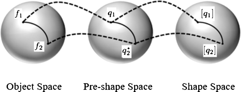
David Kendall [10] provided one of the earliest formal mathematical frameworks for quantifying shapes. In this framework we start with a finite set of points, termed landmarks, that represent an object and removes the effects of certain transformation groups, namely rigid motions and global scaling, to reach final shape representations. As depicted in Fig. 11.1, the key idea is to remove two groups via preprocessing—remove translation group by centering landmarks and remove size group by rescaling landmark vector—and reach a constrained space called the preshape space. The remaining transformation, the rotation in this case, is removed by forming orbits under this group action, or equivalence classes, and imposing a metric on this quotient space of orbits. We introduce the concepts of equivalence relations, group actions, orbits, and quotient spaces in the Appendix. A number of prominent researchers have subsequently developed this framework into a rich set of statistical tools for practical data analysis [3,17,11,6].
One of the most important challenges in shape analysis is registration. Registration stands for densely matching points across objects and using this registration for comparing shapes and developing shape models. Historically, some approaches presume that objects are already perfectly registered, whereas some other approaches use off-the-shelf methods to preregister before applying their own shape analysis. Whereas a presumption of perfect registration is severely restrictive, the use of registration as a preprocessing step is also questionable, especially when the metrics for registration have no bearing on the metrics used in ensuing shape analysis and modeling. A better solution, one that has gained recognition over the last few years, is an approach called elastic shape analysis. Here we incorporate a solution for performing registration along with the process of shape comparisons, thus resulting in a unified framework for registration, shape comparisons, and analysis. The key idea here is to endow the shape space with an elastic Riemannian metric that has an appropriate invariance under the action of the registration group (and other nuisance groups). Whereas such elastic metrics are somewhat complicated to be of use directly, especially for analyzing large datasets, there is often a square-root transformation that simplifies them into the standard Euclidean metric. This point of view is the main theme of this chapter.
In this chapter we focus on the problem of shape analysis of curves in Euclidean spaces and provide an overview of this problem area. This setup includes, for example, shape analysis of planar curves that form silhouettes of objects in images or shape analysis of space curves representing complex biomolecular structures, such as proteins and chromosomes. A particular case of this problem is when we restrict to curves in R![]() , that is, we analyze shapes of real-valued functions on a fixed interval. This fast growing area in statistics, called functional data analysis [16], deals with modeling and analyzing data, where observations are functions over intervals. The use of elastic Riemannian metrics and square-root transformations for curves was first proposed by [22,23] although this treatment used complex arithmetic and was restricted to planar curves. Later on, [15] presented a family of elastic metrics that allowed for different levels of elasticity in shape comparisons. Joshi et al. [9] and Srivastava et al. [19] introduced a square-root representation, slightly different from that of Younes, which was applicable to curves in any Euclidean space. Subsequently, several other elastic metrics and square-root representations, each representing a different strength and limitation, have been discussed in the literature [25,1,2,12,24]. In this chapter we focus on the framework of [9] and [19] and demonstrate that approach using a number of examples involving functional and curve data.
, that is, we analyze shapes of real-valued functions on a fixed interval. This fast growing area in statistics, called functional data analysis [16], deals with modeling and analyzing data, where observations are functions over intervals. The use of elastic Riemannian metrics and square-root transformations for curves was first proposed by [22,23] although this treatment used complex arithmetic and was restricted to planar curves. Later on, [15] presented a family of elastic metrics that allowed for different levels of elasticity in shape comparisons. Joshi et al. [9] and Srivastava et al. [19] introduced a square-root representation, slightly different from that of Younes, which was applicable to curves in any Euclidean space. Subsequently, several other elastic metrics and square-root representations, each representing a different strength and limitation, have been discussed in the literature [25,1,2,12,24]. In this chapter we focus on the framework of [9] and [19] and demonstrate that approach using a number of examples involving functional and curve data.
We mention in passing that such elastic frameworks have also been developed for curves taking values on nonlinear domains also, including unit spheres [26], hyperbolic spaces [5,4], the space of symmetric positive definite matrices [27], and some other manifolds. Additionally, elastic metrics and square-root representations have also been used to analyze shapes of surfaces in R3![]() . These methods provide techniques for registration of points across objects, as well as comparisons of their shapes, in a unified metric-based framework. For details, we refer the reader to a text book by [8] and some related papers [7,21,13].
. These methods provide techniques for registration of points across objects, as well as comparisons of their shapes, in a unified metric-based framework. For details, we refer the reader to a text book by [8] and some related papers [7,21,13].
11.2 Registration problem and elastic approach
Using a formulation similar to Kendall's approach, we provide a comprehensive framework for comparing shapes of curves in Euclidean spaces. The key idea here is to study curves as (continuous) parameterized objects and to use parameterization as a tool for registration of points across curves. Consequently, this introduces an additional group, namely the re-parameterization group, which is added in the representation and needs to be removed using the notion of equivalence class and quotient spaces.
11.2.1 The L2 norm and associated problems
As mentioned earlier, the problem of registration of points across curves is important in comparisons of shapes of curves. To formalize this problem, let Γ represent all boundary-preserving diffeomorphisms of [0,1]![]() to itself. Elements of Γ play the role of re-parameterization (and registration) functions. Let F
to itself. Elements of Γ play the role of re-parameterization (and registration) functions. Let F![]() be the set of all absolutely continuous parameterized curves of the type f:[0,1]→Rn
be the set of all absolutely continuous parameterized curves of the type f:[0,1]→Rn![]() . For any f∈F
. For any f∈F![]() and γ∈Γ
and γ∈Γ![]() , the composition f∘γ
, the composition f∘γ![]() denotes a reparameterization of f. Note that both f and f∘γ
denotes a reparameterization of f. Note that both f and f∘γ![]() go through the same set of points in Rn
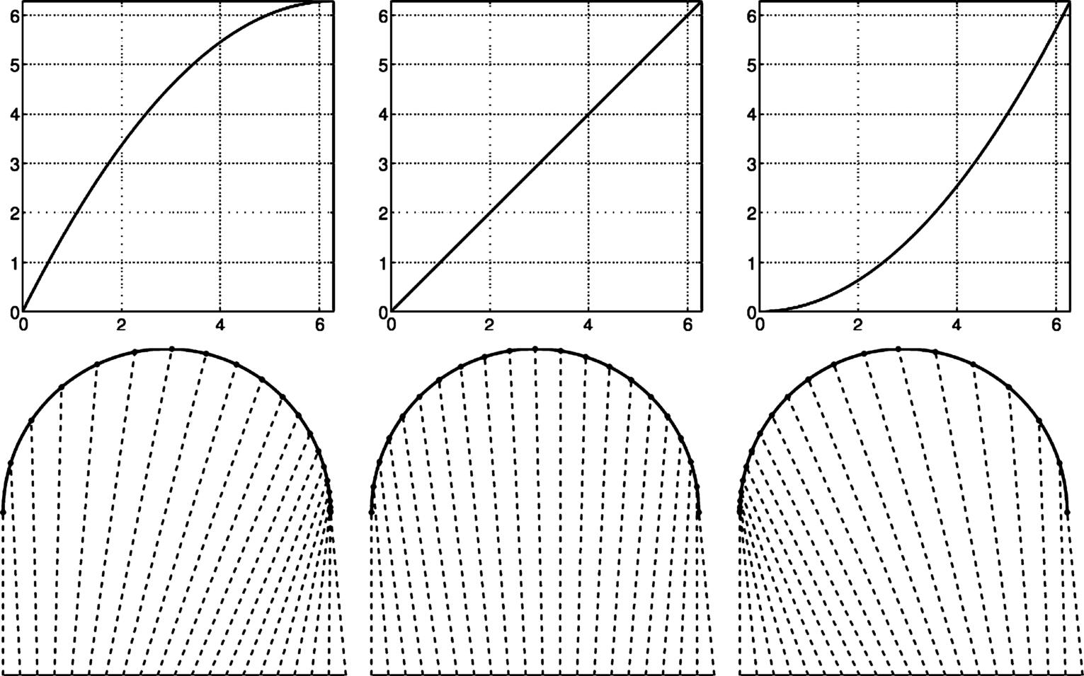
go through the same set of points in Rn![]() and thus have exactly the same shape. Fig. 11.2 shows an example of reparameterization of a semicircular curve f. The top row shows three γ's, and the bottom row shows the corresponding parameterizations of f. For any t∈[0,1]
and thus have exactly the same shape. Fig. 11.2 shows an example of reparameterization of a semicircular curve f. The top row shows three γ's, and the bottom row shows the corresponding parameterizations of f. For any t∈[0,1]![]() and any two curves f1,f2∈F
and any two curves f1,f2∈F![]() , the points f1(t)
, the points f1(t)![]() and f2(t)
and f2(t)![]() are said to be registered to each other. If we re-parameterize f2
are said to be registered to each other. If we re-parameterize f2![]() by γ, then the registration of f1(t)
by γ, then the registration of f1(t)![]() changes to f2(γ(t))
changes to f2(γ(t))![]() for all t. In this way the reparameterization γ controls registration of points between f1
for all t. In this way the reparameterization γ controls registration of points between f1![]() and f2
and f2![]() . On one hand, reparameterization is a nuisance variable since it preserves the shape of a curve but, and on the other hand, it is an important tool in controlling registration between curves.
. On one hand, reparameterization is a nuisance variable since it preserves the shape of a curve but, and on the other hand, it is an important tool in controlling registration between curves.
To register two curves, we need an objective function that evaluates and quantifies the level of registration between them. A natural choice will use the L2![]() norm, but it has some unexpected pitfalls as described next. Let ‖f‖
norm, but it has some unexpected pitfalls as described next. Let ‖f‖![]() represent the L2
represent the L2![]() norm, that is, ‖f‖=√∫10|f(t)|2dt
norm, that is, ‖f‖=√∫10|f(t)|2dt![]() , of a curve f, where |⋅|
, of a curve f, where |⋅|![]() inside the integral denotes the ℓ2
inside the integral denotes the ℓ2![]() norm of a vector. The L2
norm of a vector. The L2![]() norm provides the most commonly used Hilbert structure in functional data analysis. Despite its popularity, there are problems with this metric. The main problem is that as an objective function for registration, it leads to a degeneracy, called the pinching effect. In other words, if we try to minimize ‖f1−f2∘γ‖
norm provides the most commonly used Hilbert structure in functional data analysis. Despite its popularity, there are problems with this metric. The main problem is that as an objective function for registration, it leads to a degeneracy, called the pinching effect. In other words, if we try to minimize ‖f1−f2∘γ‖![]() over γ, this quantity can be made infinitesimally small despite f1
over γ, this quantity can be made infinitesimally small despite f1![]() and f2
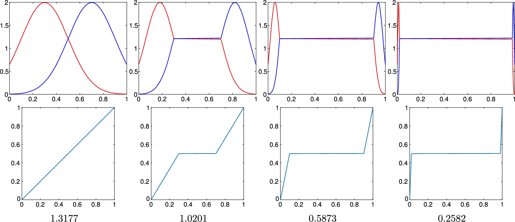
and f2![]() being very different functions. Fig. 11.3 shows a simple example to illustrate this idea using scalar functions on [0,1]
being very different functions. Fig. 11.3 shows a simple example to illustrate this idea using scalar functions on [0,1]![]() . The top left panel of the figure shows to functions f1
. The top left panel of the figure shows to functions f1![]() , f2
, f2![]() that agree at only one point t=0.5
that agree at only one point t=0.5![]() in the domain. We design a sequence of piecewise-linear time-warping functions γs (shown in the bottom row) that increasingly spend time at t=0.5
in the domain. We design a sequence of piecewise-linear time-warping functions γs (shown in the bottom row) that increasingly spend time at t=0.5![]() from left to right, resulting in the steady decrease in the L2
from left to right, resulting in the steady decrease in the L2![]() norm ‖f1∘γ−f2∘γ‖
norm ‖f1∘γ−f2∘γ‖![]() . Continuing this process, we can arbitrarily decrease the L2
. Continuing this process, we can arbitrarily decrease the L2![]() norm between two functions, irrespective of the other values of these functions. Thus an optimization problem of the type infγ∈Γ‖f1−f2∘γ‖
norm between two functions, irrespective of the other values of these functions. Thus an optimization problem of the type infγ∈Γ‖f1−f2∘γ‖![]() has degenerate solutions. This problem is well recognized in the literature [16,14], and the most common solution used to avoid pinching is to penalize large warpings using roughness penalties. More precisely, we solve an optimization problem of the type
has degenerate solutions. This problem is well recognized in the literature [16,14], and the most common solution used to avoid pinching is to penalize large warpings using roughness penalties. More precisely, we solve an optimization problem of the type
infγ∈Γ(‖f1−f2∘γ‖2+λR(γ)),
where R(γ)![]() measures the roughness of γ. Examples of R
measures the roughness of γ. Examples of R![]() include ∫˙γ(t)2dt
include ∫˙γ(t)2dt![]() , ∫¨γ(t)2dt
, ∫¨γ(t)2dt![]() , and so on. The role of R
, and so on. The role of R![]() is to discourage large time warpings. By large we mean γs whose first or second derivatives have high norms.
is to discourage large time warpings. By large we mean γs whose first or second derivatives have high norms.
 norm between them. In each column we show f1∘γ, f2∘γ (top panel), γ (bottom panel), and the value of ‖f1∘γ − f2∘γ‖ below them.
Whereas this solution helps avoid the pinching effect, it often also restricts alignment of functions. Since it reduces the solution space for warping functions, it can also inhibit solutions that correctly require large deformations. Fig. 11.4 shows an example of this problem using two functions f1![]() and f2
and f2![]() shown in the top left panel. In this example we use the first order penalty (∫˙γ(t)2dt
shown in the top left panel. In this example we use the first order penalty (∫˙γ(t)2dt![]() ) in Eq. (11.1) and study several properties of the resulting solution—does to align the functions well, is the solution symmetric in the functions f1
) in Eq. (11.1) and study several properties of the resulting solution—does to align the functions well, is the solution symmetric in the functions f1![]() and f2
and f2![]() , does it have pinching effect, and how sensitive is the solution to the choice of λ? In each row, for a certain value of λ, we first obtain an optimal value of γ in Eq. (11.1). Then, to study the symmetry of the solution, we swap f1
, does it have pinching effect, and how sensitive is the solution to the choice of λ? In each row, for a certain value of λ, we first obtain an optimal value of γ in Eq. (11.1). Then, to study the symmetry of the solution, we swap f1![]() and f2
and f2![]() and solve this optimization again. Finally, we compose the two resulting optimal warping functions. If the composition is a perfect identity function γid(t)=t
and solve this optimization again. Finally, we compose the two resulting optimal warping functions. If the composition is a perfect identity function γid(t)=t![]() , then the solution is called inverse consistent (and symmetric), otherwise not. In the first row, where λ=0
, then the solution is called inverse consistent (and symmetric), otherwise not. In the first row, where λ=0![]() , we see that the solution is inverse consistent, but there is substantial pinching, as expected. As we increase λ (shown in the second row), the level of pinching is reduced, but the solution also shows a small inconsistency in the forward and backward solutions. In the last row, where λ is large, the pinching effect is gone, but inverse inconsistency has increased. Also, due to increased penalty, the quality of alignment has gone down too. This discussion also points an obvious limitation of methods involving penalty terms. We need to decide which type of penalty and how large λ should be used in real situations. In contrast to the penalized L2
, we see that the solution is inverse consistent, but there is substantial pinching, as expected. As we increase λ (shown in the second row), the level of pinching is reduced, but the solution also shows a small inconsistency in the forward and backward solutions. In the last row, where λ is large, the pinching effect is gone, but inverse inconsistency has increased. Also, due to increased penalty, the quality of alignment has gone down too. This discussion also points an obvious limitation of methods involving penalty terms. We need to decide which type of penalty and how large λ should be used in real situations. In contrast to the penalized L2![]() approach, the elastic approach described in this chapter results in the solution shown in the bottom row. This solution is inverse consistent, rules out the pinching effect (and does not need any penalty or choice of λ), and achieves an excellent registration between the functions. Additionally, the computational cost is very similar to the penalized L2
approach, the elastic approach described in this chapter results in the solution shown in the bottom row. This solution is inverse consistent, rules out the pinching effect (and does not need any penalty or choice of λ), and achieves an excellent registration between the functions. Additionally, the computational cost is very similar to the penalized L2![]() approach.
approach.
 norm in registering functions using time warpings: pinching effect, asymmetry of solutions, and need to balance matching with penalty. The bottom row shows the proposed method that avoids all three problems.
Lack of invariance under L2![]() norm To study the shape of curves, we need representations and metrics that are invariant to rigid motions, global scale, and reparameterization of curves. The biggest challenge comes from the last group since it is an infinite-dimensional group and requires closer inspection. To understand this issue, take an analogous task of removing the rotation group in Kendall's shape analysis, where each object is represented by a set of landmarks. Let X1,X2∈Rn×k
norm To study the shape of curves, we need representations and metrics that are invariant to rigid motions, global scale, and reparameterization of curves. The biggest challenge comes from the last group since it is an infinite-dimensional group and requires closer inspection. To understand this issue, take an analogous task of removing the rotation group in Kendall's shape analysis, where each object is represented by a set of landmarks. Let X1,X2∈Rn×k![]() represent two sets of landmarks (k landmarks in Rn
represent two sets of landmarks (k landmarks in Rn![]() ), and let SO(n)
), and let SO(n)![]() be the set of all rotations in Rn
be the set of all rotations in Rn![]() . To (rotationally) align X2
. To (rotationally) align X2![]() to X1
to X1![]() , we solve for a Procrustes rotation according to argminO∈SO(n)‖X1−OX2‖F
, we solve for a Procrustes rotation according to argminO∈SO(n)‖X1−OX2‖F![]() , where ‖⋅‖F
, where ‖⋅‖F![]() denotes the Frobenius norm of matrices. In other words, we keep X1
denotes the Frobenius norm of matrices. In other words, we keep X1![]() fixed and rotate X2
fixed and rotate X2![]() into a configuration that minimizes the Frobenius norm between them. The choice of Frobenius norm is important because it satisfies the following property:
into a configuration that minimizes the Frobenius norm between them. The choice of Frobenius norm is important because it satisfies the following property:
‖X1−X2‖=‖OX1−OX2‖for allX1,X2∈Rn×k,O∈SO(n).
If this property was not satisfied, we would not be able to perform Procrustes rotation. In mathematical terms we say that the action of SO(n)![]() on Rn×k
on Rn×k![]() is by isometries under the Frobenius norm or that the metric is invariant under the rotation group action. (Please refer to the Appendix for a proper definition of isometry under group actions.) A similar approach is needed for performing registration and removing the reparameterization group in the case of functions and curves. However, it is easy to see that ‖f1−f2‖≠‖f1∘γ−f2∘γ‖
is by isometries under the Frobenius norm or that the metric is invariant under the rotation group action. (Please refer to the Appendix for a proper definition of isometry under group actions.) A similar approach is needed for performing registration and removing the reparameterization group in the case of functions and curves. However, it is easy to see that ‖f1−f2‖≠‖f1∘γ−f2∘γ‖![]() in general. In fact, Fig. 11.3 already provides an example of this inequality. Since L2
in general. In fact, Fig. 11.3 already provides an example of this inequality. Since L2![]() norm is not preserved under identical reparameterizations of curves, it is not suitable for use in registration and shape analysis. Thus we seek a new metric to accomplish registration and shape analysis of curves.
norm is not preserved under identical reparameterizations of curves, it is not suitable for use in registration and shape analysis. Thus we seek a new metric to accomplish registration and shape analysis of curves.
11.2.2 SRVFs and curve registration
Now we describe an elastic approach that addresses these issues and provides a fundamental tool for registration and shape analysis of curves.
As earlier, let F![]() be the set of all absolutely continuous parameterized curves in Rn
be the set of all absolutely continuous parameterized curves in Rn![]() , and let Γ be the same of all reparameterization functions. Define the square-root velocity function (SRVF) [19,18] of f as a mathematical representation of f given by
, and let Γ be the same of all reparameterization functions. Define the square-root velocity function (SRVF) [19,18] of f as a mathematical representation of f given by
q(t)={˙f(t)√|˙f(t)|,|˙f(t)|≠0,0,|˙f(t)|=0.
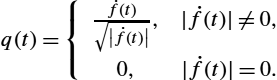
In case of n=1![]() this expression simply reduces to q(t)=sign(˙f(t))×√|˙f(t)|
this expression simply reduces to q(t)=sign(˙f(t))×√|˙f(t)|![]() . Here are some important properties associated with this definition.
. Here are some important properties associated with this definition.
- • If f is absolutely continuous, as assumed, then q is square integrable, that is, ‖q‖<∞
 .
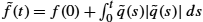
. - • This transformation from f to q is invertible up to a constant, with the inverse given by f(t)=f(0)+∫t0q(s)|q(s)|ds
 . In fact the mapping f↦(f(0),q)
 is a bijection between F
 and R×L2([0,1],Rn)
 .
. - • If f is reparameterized by γ∈Γ
 to result in f∘γ
 , the SRVF change from q to (q∘γ)√˙γΔ=(q⋆γ)
 . In other words, the action of Γ on L2 is given by q⋆γ
 . Also, if a curve is rotated by a matrix O∈SO(n)
 , then its SRVF gets rotated by the same matrix O, that is, the SRVF of a curve Of is given by Oq.
 - • The length of the curve f, given by L[f]=∫10|˙f(t)|dt
 , is equal to the L2 norm of its SRVF q, that is, L[f]=‖q‖
 .
. - • The most important property of this representation is preservation of the L2 norm under time warping or reparameterization, that is,
‖q1−q2‖=‖(q1⋆γ)−(q2⋆γ)‖,∀q1,q2∈L2([0,1],Rn),γ∈Γ.
- We already know that L2 norm is preserved under identical rotation, that is, ‖q1−q2‖=‖Oq1−Oq2‖
 .
.
In view of the invariant property, this representation provides a proper setup for registration of functional and curve data.
Definition 11.1
Pairwise registration
We make a few remarks about this registration formulation.
- 1. No Pinching: Firstly, this setup does not have any pinching problem. A special case of the isometry condition is that ‖q⋆γ‖=‖q‖
 for all q and γ. In other words, the action of Γ on L2 is norm preserving. Thus pinching is not possible in this setup.
 - 2. No Need for a Penalty Term: Since there is no pinching, we do not have to include any penalty term in this setup. Therefore there is no inherent problem about choosing the relative weight between the data term and the penalty term. However, if we need to control the time warping or registration, beyond the basic formulation, we can still add an additional penalty term as desired.
- 3. Inverse Symmetry: As stated in Eq. (11.5), the registration of f1
 to f2
to f2 results in the same solution as the registration of f2 to f1. The equality between the two terms in that equation comes from fact that SO(n)
 and Γ are groups, and the isometry condition is satisfied (Eq. (11.4)).
 - 4. Invariance to Scale and Translation: We can show that the optimizer in Eq. (11.5) does not change if either function is changed using positive scaling or translation, that is, we can replace any fi(t)
 with afi(t)+c
 for any a∈R+
 and c∈Rn
 , and the solution does not change. This is an important requirement for shape analysis since shape is invariant to these transformations. The solution is invariant to translation because the SRVF qi
 is based on the of the curve fi
 and because
arginfγ∈Γ‖q1−(q2⋆γ)‖=arginfγ∈Γ‖a1q1−a2(q2⋆γ)‖
- for any a1,a2∈R+
 .
. - 5. Proper Metric: As described in the next section, the infimum in Eq. (11.5) is a proper metric itself in a quotient space and hence can be used for ensuing statistical analysis. (Please refer to the definition of a metric on the quotient space M/G
 using an invariant metric on parent space M).
In Eq. (11.5) the optimization over SO(n)![]() is performed using the Procrustes solution:
is performed using the Procrustes solution:
O⁎={UVif det(A)>0,U[100−1]VTotherwise,
where A=∫10q1(t)qT2(t)dt∈Rn×n![]() , and svd(A)=UΣVT
, and svd(A)=UΣVT![]() . The optimization over Γ is accomplished using the dynamic programming algorithm [20]. The optimization over SO(n)×Γ
. The optimization over Γ is accomplished using the dynamic programming algorithm [20]. The optimization over SO(n)×Γ![]() is performed by iterating between the two individual solutions until convergence.
is performed by iterating between the two individual solutions until convergence.
We present some examples of registration of functions and curves to illustrate this approach. In the case n=1![]() we do not have any rotation in Eq. (11.5), and one minimizes only over Γ using the dynamic programming algorithm. The last row of Fig. 11.4 shows alignment of two functions studied in that example. It shows alignments of the two functions to each other and the composition of the two γ functions resulting in a perfect identity function (confirming inverse consistency). Note that even though the optimization is performed using SRVFs in L2
we do not have any rotation in Eq. (11.5), and one minimizes only over Γ using the dynamic programming algorithm. The last row of Fig. 11.4 shows alignment of two functions studied in that example. It shows alignments of the two functions to each other and the composition of the two γ functions resulting in a perfect identity function (confirming inverse consistency). Note that even though the optimization is performed using SRVFs in L2![]() space, the results are displayed in the original function space for convenience. Fig. 11.5 shows another example of registering functions using this approach.
space, the results are displayed in the original function space for convenience. Fig. 11.5 shows another example of registering functions using this approach.

Fig. 11.6 shows a few examples of registration of points along planar curves. In each panel we show the two curves in red (light gray in print version) and blue (dark gray in print version), and optimal correspondences across these curves using black lines, obtained using Eq. (11.5). We can see that the algorithm is successful in matching points with similar geometric features (local orientation, curvature, etc.) despite different locations of matched points along the two curves. This success in registering curves translates into a superior performance in ensuing shape analysis.

11.3 Shape space and geodesic paths
So far we have focused on an important problem of registering curves and functions. Our larger goal, of course, is the shape analysis of these objects, and registration plays an important role in that analysis. Returning to the problem of analyzing shapes, we describe the framework for an elastic shape analysis of Euclidean curves. It is called elastic because it incorporates the registration of curves as a part of their shape comparisons.
This framework follows the approach laid out in Fig. 11.1. We will use the SRVF representation of curves, reach a preshape space by removing some nuisance transformations, and form quotient space of that preshape space under the remaining nuisance transformations. Once again, let F![]() be the set of all absolutely continuous curves in Rn
be the set of all absolutely continuous curves in Rn![]() , and let L2
, and let L2![]() denote the set of square-integrable curves in Rn
denote the set of square-integrable curves in Rn![]() . For any f∈F
. For any f∈F![]() , its length L[f]=‖q‖
, its length L[f]=‖q‖![]() , where q is the SRVF of f. So, if we rescale f to be of unit length, then its SRVF satisfies ‖q‖=1
, where q is the SRVF of f. So, if we rescale f to be of unit length, then its SRVF satisfies ‖q‖=1![]() . Let C
. Let C![]() denote the unit Hilbert sphere inside L2
denote the unit Hilbert sphere inside L2![]() . C
. C![]() is called the preshape space and is the set of SRVFs representing all unit length curves in F
is called the preshape space and is the set of SRVFs representing all unit length curves in F![]() . The geometry of C
. The geometry of C![]() is simple, and we can compute distances/geodesics on C
is simple, and we can compute distances/geodesics on C![]() relatively easily. For any two points q1,q2∈C
relatively easily. For any two points q1,q2∈C![]() , the distance between them on C
, the distance between them on C![]() is given by the arc length dc(q1,q2)=cos−1(〈q1,q2〉)
is given by the arc length dc(q1,q2)=cos−1(〈q1,q2〉)![]() . The geodesic path between them is the shorter arc on a great circle given by
. The geodesic path between them is the shorter arc on a great circle given by
α:[0,1]→C,α(τ)=1sinθ(sin((1−τ)θ)q1+sin(τθ)q2),
where θ=dc(q1,q2)![]() .
.
In representing a unit-length f∈F![]() by its q∈C
by its q∈C![]() we have removed its translation (since q depends only on the derivatives of f) and its scale. However, the rotation and re-parameterization variabilities are still left in this representation, that is, we can have two curves with exactly the same shape but at different rotations and reparameterizations and thus with nonzero distance between them in C
we have removed its translation (since q depends only on the derivatives of f) and its scale. However, the rotation and re-parameterization variabilities are still left in this representation, that is, we can have two curves with exactly the same shape but at different rotations and reparameterizations and thus with nonzero distance between them in C![]() . These transformations are removed using groups actions and equivalence relations, as described next. For any O∈SO(n)
. These transformations are removed using groups actions and equivalence relations, as described next. For any O∈SO(n)![]() and γ∈Γ
and γ∈Γ![]() , O(f∘γ)
, O(f∘γ)![]() has the same shape as f. In the SRVF representation we characterize these transformations as actions of product group SO(n)×Γ
has the same shape as f. In the SRVF representation we characterize these transformations as actions of product group SO(n)×Γ![]() on C
on C![]() according to
according to
(SO(n)×Γ)×L2→L2,(O,γ)⁎q=O(q⋆γ).
This leads to the definition of orbits or equivalent classes:
[q]={O(q⋆γ)|O∈SO(n),γ∈Γ}.
Each orbit [q]![]() represents a unique shape of curves. The set of all such orbits forms the shape space of curves
represents a unique shape of curves. The set of all such orbits forms the shape space of curves
S=C/(SO(n)×Γ)={[q]|q∈C}.
(Once again, we advise the reader not familiar with these ideas to follow the definitions given in the Appendix.)
Definition 11.2
Shape metric
The interesting part of this definition is that the process of registration of points across shapes is incorporated in the definition of shape metric. The two computations, registration of curves and comparisons of their shapes, have been unified under the same metric. The optimal deformation from one shape to the other is mathematically realized as a geodesic in the shape space. We can evaluate the geodesic between the shapes [q1]![]() and [q2]
and [q2]![]() in S
in S![]() by constructing the shortest geodesic between the two orbits in C
by constructing the shortest geodesic between the two orbits in C![]() . If (ˆO,ˆγ)
. If (ˆO,ˆγ)![]() denote the optimal arguments in Eq. (11.8), then this geodesic is given by
denote the optimal arguments in Eq. (11.8), then this geodesic is given by
α(τ)=1sinθ(sin((1−τ)θ)q1+sin(τθ)ˆq2),ˆq2=ˆO(q2⁎ˆγ).
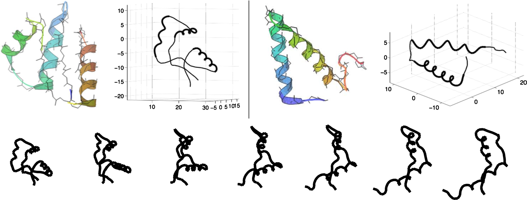
We present some examples of this framework. Fig. 11.7 shows three examples of geodesic paths between given 2D curves. It is clear from these examples that the elastic registration of points across the two curves result in a very natural deformation between them. Similar geometric parts are matched to each other despite different relative sizes across the objects, a clear depiction of stretching and compression needed for optimal matching. Fig. 11.8 shows an example of elastic geodesic between two very simple proteins viewed as curves in R3![]() .
.

Shape spaces of closed curves In case we are interested in shapes of closed curves, we need to restrict to the curves satisfying the condition f(0)=f(1)![]() . In this case it is often more natural to choose the domain of parameterization to be S1
. In this case it is often more natural to choose the domain of parameterization to be S1![]() , instead of [0,1]
, instead of [0,1]![]() . Thus Γ now represents all orientation-preserving diffeomorphisms of S1
. Thus Γ now represents all orientation-preserving diffeomorphisms of S1![]() to itself. Under the SRVF representation of f, the closure condition is given by ∫S1q(t)|q(t)|dt=0
to itself. Under the SRVF representation of f, the closure condition is given by ∫S1q(t)|q(t)|dt=0![]() . The preshape space for unit-length closed curves is
. The preshape space for unit-length closed curves is
Cc={q∈L2(S1,Rn)|∫S1|q(t)|dt=1,∫S1q(t)|q(t)|dt=0}⊂C.
An orbit or an equivalence class is defined to be: for q∈Cc![]() , [q]={O(q⋆γ)|O∈SO(n),γ∈Γ}
, [q]={O(q⋆γ)|O∈SO(n),γ∈Γ}![]() , and the resulting shape space is Sc=Cc/(SO(n)×Γ)={[q]|q∈Cc}
, and the resulting shape space is Sc=Cc/(SO(n)×Γ)={[q]|q∈Cc}![]() . The computation of geodesic paths in Cc
. The computation of geodesic paths in Cc![]() is more complicated as there is no analytical expression similar to Eq. (11.6) is available for Cc
is more complicated as there is no analytical expression similar to Eq. (11.6) is available for Cc![]() . In this case we use a numerical approximation, called path straightening [19], for computing geodesics and geodesic distances. Let dc(q1,q2)
. In this case we use a numerical approximation, called path straightening [19], for computing geodesics and geodesic distances. Let dc(q1,q2)![]() denote the length of a geodesic path in Cc
denote the length of a geodesic path in Cc![]() between any two curves q1,q2∈Cc
between any two curves q1,q2∈Cc![]() . Then the distance between their shapes is given by
. Then the distance between their shapes is given by
ds([q1],[q2])=infO∈SO(n),γ∈Γdc(q1,O(q2⋆γ)).
Fig. 11.9 shows some examples of geodesic between curves taken from the MPEG7 shape dataset.

 .
.11.4 Statistical summaries and principal modes of shape variability
Using the mathematical platform developed so far, we can define and compute several quantities that are useful in statistical shape analysis. For example, we can use the shape metric to define and compute a mean or a median shape, as a representative of shapes denoting a population. Furthermore, using the tangent structure of the shape space, we can compute principal modes for variability in a given sample of data. Given mean and covariance estimates, we can characterize underlying shape populations using Gaussian-type distributions on shape spaces.
Definition 11.3
Intrinsic, Fréchet mean

In other words, the mean is defined to be the shape that achieves minimum of the sum of squared distances to the given shapes. There is a well-known gradient-based algorithm for estimating this mean from given data.
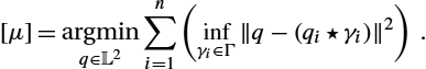
In case of real-valued functions, we can simplify the setup and use it to register and align multiple functions. The basic idea is to use a template to register all the given curves using previous pairwise alignment. A good candidate of the template is a mean function defined previously. In the case of unscaled functions the definition of the mean simplifies to
[μ]=argminq∈L2n∑i=1(infγi∈Γ‖q−(qi⋆γi)‖2).
If we fix the optimal warpings to be {γi}![]() s, then the solution for the mean reduces to μ=1nn∑i=1(qi⋆γi)
s, then the solution for the mean reduces to μ=1nn∑i=1(qi⋆γi)![]() . Using this idea, we can write an iterative algorithm for registration of multiple functions or curves.
. Using this idea, we can write an iterative algorithm for registration of multiple functions or curves.
Multiple alignment algorithm
- 1. Use Eq. (11.3) to compute SRVFs qi, i=1,…,n
 , from the given fi.
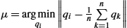
 - 2. Initialize the mean with μ=argminqi‖qi−1nn∑k=1qk‖
 .
. - 3. For each qi, solve γi=argminγ∈Γ‖μ−(qi⋆γ)‖
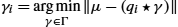 . Compute the aligned SRVFs ˜qi=(qi⋆γi)
 .
. - 4. Update μ↦1nn∑i=1˜qi
 and return to step 2 until the change ‖μ−1nn∑i=1˜qi‖
 is small.
 - 5. Map all the SRVFs back to the function space using by ˜f(t)=f(0)+∫t0˜q(s)|˜q(s)|ds
 .
.
Fig. 11.10 shows an example of registration of multiple functions using this algorithm. The left panel shows a set of simulated functions {fi}![]() that all are bimodal, but their modes differ in the locations and heights. This set forms the input to the algorithm, and the next two panels show the outputs. The middle panel shows the functions {˜fi}
that all are bimodal, but their modes differ in the locations and heights. This set forms the input to the algorithm, and the next two panels show the outputs. The middle panel shows the functions {˜fi}![]() associated with the aligned SRVFs {˜qi}
associated with the aligned SRVFs {˜qi}![]() , and the right panel shows the optimal time warping functions {γi}
, and the right panel shows the optimal time warping functions {γi}![]() . We can see the high quality of registration in matching of peaks and valleys across functions.
. We can see the high quality of registration in matching of peaks and valleys across functions.
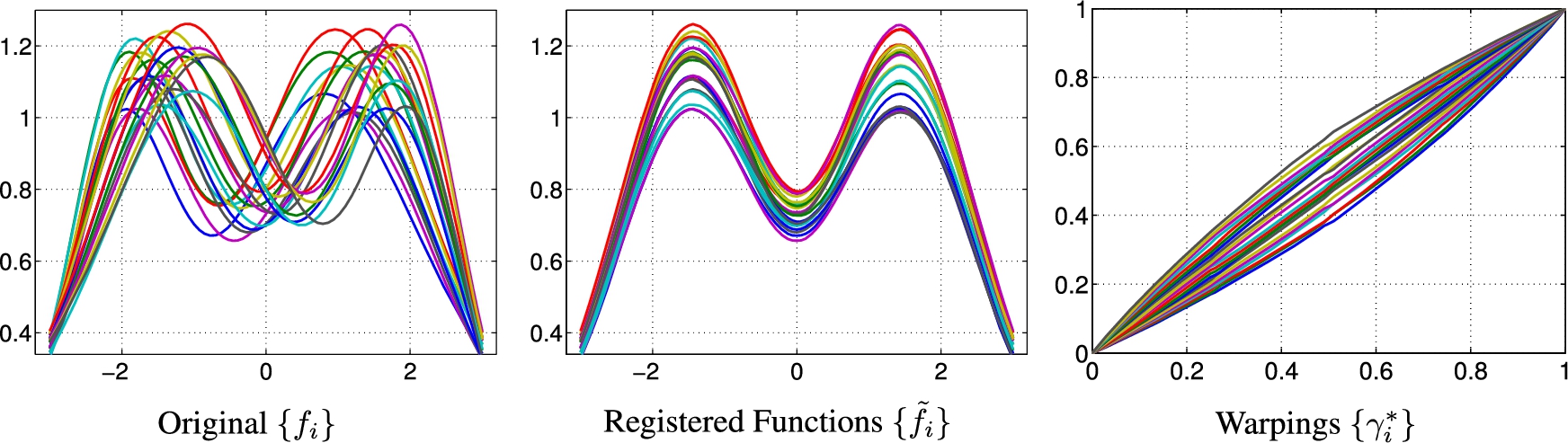
Fig. 11.11 shows some more examples of multiple function registration, this time using real data. The two rows of this figure correspond to female (top) and male (bottom) growth curves taken from the famous Berkeley growth dataset. Each curve shows the rate at which the height of an individual changes from the age of one to twelve. Each row shows the original growth rate functions {fi}![]() (left), their registrations {˜fi}
(left), their registrations {˜fi}![]() (middle), and the optimal warpings {γi}
(middle), and the optimal warpings {γi}![]() . The peaks in rate functions, denoting growth spurts, are better matched after registrations and are easier to interpret in the resulting data.
. The peaks in rate functions, denoting growth spurts, are better matched after registrations and are easier to interpret in the resulting data.
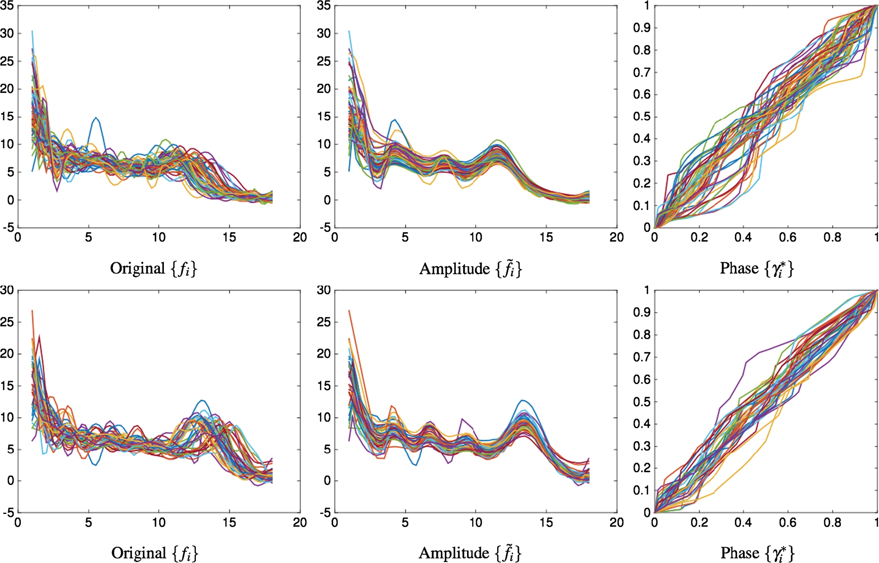
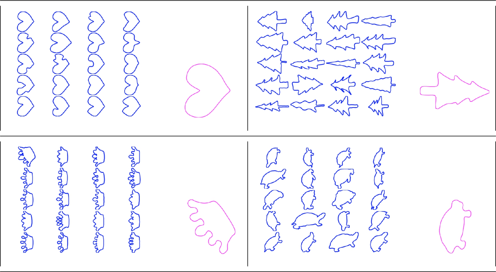
Fig. 11.12 shows some examples of mean shapes computed for a set of given shapes. We can see that the mean shapes are able to preserve main distinguishing features of the shape class while smoothing out the intraclass variabilities.
We can use the shape metric and the flatness of the tangent space to discover principal modes of variability in the given set of shapes. Let T[μ]S![]() denote the tangent space to S
denote the tangent space to S![]() at the mean shape [μ]
at the mean shape [μ]![]() , and let exp−1[μ]([q])
, and let exp−1[μ]([q])![]() denote the mapping from the shape space S
denote the mapping from the shape space S![]() to this tangent space using the inverse exponential map. We evaluate this mapping by finding the geodesic α from [μ]
to this tangent space using the inverse exponential map. We evaluate this mapping by finding the geodesic α from [μ]![]() to a shape [q]
to a shape [q]![]() and then computing the initial velocity of the geodesic, that is, exp−1[μ]([q])=˙α(0)
and then computing the initial velocity of the geodesic, that is, exp−1[μ]([q])=˙α(0)![]() . We also call these initial velocities the shooting vectors. Let vi=exp−1[μ]([qi])
. We also call these initial velocities the shooting vectors. Let vi=exp−1[μ]([qi])![]() , i=1,2,…,n
, i=1,2,…,n![]() , be the shooting vectors from the mean shape to the given shapes. Then performing PCA of {vi}
, be the shooting vectors from the mean shape to the given shapes. Then performing PCA of {vi}![]() provides the directions of maximum variability in the given shapes and can be used to visualize the main variability in that set. Fig. 11.13 shows three examples of this idea using some leaf shapes. In each panel of the top row we show the set of given leafs and their mean shapes. The bottom row shows the shape variability along the two dominant modes of variability, obtained using PCA in the tangent space. In the bottom plots the two axes represent the two dominant directions, and we can see the variation in shapes as one moves along these coordinates.
provides the directions of maximum variability in the given shapes and can be used to visualize the main variability in that set. Fig. 11.13 shows three examples of this idea using some leaf shapes. In each panel of the top row we show the set of given leafs and their mean shapes. The bottom row shows the shape variability along the two dominant modes of variability, obtained using PCA in the tangent space. In the bottom plots the two axes represent the two dominant directions, and we can see the variation in shapes as one moves along these coordinates.

11.5 Summary and conclusion
This chapter describes an elastic approach to shape analysis of curves in Euclidean spaces. It focuses on the problem of registration of points across curves and shows that the standard L2![]() norm, or its penalized version, has inferior mathematical properties and practical performances. Instead, it uses a combination of SRVFs and L2
norm, or its penalized version, has inferior mathematical properties and practical performances. Instead, it uses a combination of SRVFs and L2![]() norm to derive a framework for a unified shape analysis framework. Here we register curves and compare their shape in a single optimization framework. We compute geodesic paths, geodesic distances, and shape summarizes using the geometries of shape spaces. These tools can then be used in statistical modeling and analysis of shapes of curves.
norm to derive a framework for a unified shape analysis framework. Here we register curves and compare their shape in a single optimization framework. We compute geodesic paths, geodesic distances, and shape summarizes using the geometries of shape spaces. These tools can then be used in statistical modeling and analysis of shapes of curves.
Appendix Mathematical background
We summarize here some background knowledge of algebra and differential geometry with the example of planar shapes represented by k ordered points in R2![]() , denoted by X∈R2×k
, denoted by X∈R2×k![]() . Clearly, X and OX,O∈SO(2)
. Clearly, X and OX,O∈SO(2)![]() have the same shape. That can be defined strictly through the following concepts.
have the same shape. That can be defined strictly through the following concepts.
Definition 11.4
A binary relation ∼ on a set X is called an equivalence relation if it satisfies the following properties: For x,y,z∈X![]() ,
,
- • x∼x
 (reflexivity),
 - • x∼y⇔y∼x
 (symmetry),
 - • x∼y
 , y∼z⇒x∼y
 (transitivity).
Definition 11.5
Equivalence class. [x]={y∈X|y∼x}![]() .
.
Definition 11.6
The quotient space of X under equivalence relation ∼ is the set of all equivalence classes [x]![]() , denoted by X/∼
, denoted by X/∼![]() .
.
Thus the space of planar shapes in the form of discrete points is the quotient space of R2×k/SO(2)![]() . To measure the difference between two shapes, we need a proper metric. For R2×k
. To measure the difference between two shapes, we need a proper metric. For R2×k![]() , a natural choice is the Euclidean metric, but for a nonlinear manifold, the difference is measured by the length of the shortest path connecting the two shapes, which requires the following definitions.
, a natural choice is the Euclidean metric, but for a nonlinear manifold, the difference is measured by the length of the shortest path connecting the two shapes, which requires the following definitions.
Definition 11.7
A Riemannian metric on differential manifold M is a smooth inner product on the tangent Tp(M)![]() space of M. A differential manifold with a Riemannian metric is called Riemannian manifold.
space of M. A differential manifold with a Riemannian metric is called Riemannian manifold.
Definition 11.8
Let α:[0,1]→M![]() represent a path on a Riemannian manifold M. Then dαdt
represent a path on a Riemannian manifold M. Then dαdt![]() represents the velocity at time t. The length of α can be defined as L[α]=∫10√〈dαdt,dαdt〉dt
represents the velocity at time t. The length of α can be defined as L[α]=∫10√〈dαdt,dαdt〉dt![]() . The path connecting two points with shortest length is called the geodesic between them. The length of geodesic is a proper metric between the two points.
. The path connecting two points with shortest length is called the geodesic between them. The length of geodesic is a proper metric between the two points.
Example 11.1
The geodesic between p,q∈Rn![]() is a straight line: α(τ)=(1−τ)p+τq
is a straight line: α(τ)=(1−τ)p+τq![]() , τ∈[0,1]
, τ∈[0,1]![]() .
.
Example 11.2
The geodesic between p,q∈Sn⊆Rn+1![]() is the arc on a great circle: α(τ)=1sinθ[sin((1−τ)θ)p+sin(τθ)q]
is the arc on a great circle: α(τ)=1sinθ[sin((1−τ)θ)p+sin(τθ)q]![]() , τ∈[0,1]
, τ∈[0,1]![]() .
.
For X∈R2×k![]() , the fact ‖X‖=‖OX‖
, the fact ‖X‖=‖OX‖![]() , O∈SO(2)
, O∈SO(2)![]() , induces two important concepts, group action and isometry.
, induces two important concepts, group action and isometry.
Definition 11.9
A Lie group G is a smooth manifold such that the group operations G→G×G![]() defined by (g,h)→gh
defined by (g,h)→gh![]() and G→G
and G→G![]() defined by g→g−1
defined by g→g−1![]() are both smooth mappings.
are both smooth mappings.
The groups appearing in this chapter are all Lie groups.
Definition 11.10
Given a manifold M and a Lie group G, a left group action of G on M is a map G×M→M![]() , denoted by (g,p)
, denoted by (g,p)![]() , satisfying
, satisfying
- 1. (g1,(g2,p))=((g1⋅g2),p)
 , ∀g1,g2∈G
 and p∈M
 .
. - 2. (e,p)=p
 , ∀p∈M
 .
.
Similarly, we can define the right group action.
Definition 11.11
Given two metric spaces X and Y, a map f:X→Y![]() is called an isometry or distance preserving if dX(a,b)=dY(f(a),f(b))
is called an isometry or distance preserving if dX(a,b)=dY(f(a),f(b))![]() for all a,b∈X
for all a,b∈X![]() .
.
Definition 11.12
A group action of G on a Riemannian manifold M is called isometric if it preserves the Riemannian metric on M, that is, d(x,y)=d((g,x),(g,y))![]() for all g∈G
for all g∈G![]() and x,y∈M
and x,y∈M![]() .
.
Definition 11.13
Given a manifold M, for any p∈M![]() , the orbit of p under the action of group G is defined as [p]={g⋅p|g∈G}
, the orbit of p under the action of group G is defined as [p]={g⋅p|g∈G}![]() .
.
Example 11.3
The rotation group SO(n)![]() acts on Rn
acts on Rn![]() by the action O⁎x=Ox
by the action O⁎x=Ox![]() for all O∈SO(n)
for all O∈SO(n)![]() and x∈Rn
and x∈Rn![]() . The orbit of x is the sphere centered at the origin with radius ‖x‖
. The orbit of x is the sphere centered at the origin with radius ‖x‖![]() .
.
For a planar shape denoted by a 2×k![]() matrix X, the shape can be identified by an orbit [X]={OX|O∈SO(2)}
matrix X, the shape can be identified by an orbit [X]={OX|O∈SO(2)}![]() .
.
Definition 11.14
For group G acting on the manifold M, the quotient space M/G![]() is defined as the set of all orbits of G in M: M/G={[p]|p∈M}
is defined as the set of all orbits of G in M: M/G={[p]|p∈M}![]() .
.
Definition 11.15
We illustrate this idea by an example. Let R2×k![]() be the space of planar shapes of k points with Euclidean metric. Consider the action of rotation group SO(2)
be the space of planar shapes of k points with Euclidean metric. Consider the action of rotation group SO(2)![]() on R2×k
on R2×k![]() . The metric on the quotient space R2×k/SO(2)
. The metric on the quotient space R2×k/SO(2)![]() is
is
dR2×k/SO(2)([X1],[X2])=minO∈SO(2)‖X1−OX2‖.
The geodesic between two shapes [X1]![]() and [X2]
and [X2]![]() is α(τ)=(1−τ)X1+τO⁎X2
is α(τ)=(1−τ)X1+τO⁎X2![]() , where O⁎=argminO∈SO(2)‖X1−OX2‖
, where O⁎=argminO∈SO(2)‖X1−OX2‖![]() , τ∈[0,1]
, τ∈[0,1]![]() . If the two shapes are rescaled to be unit length, that is, ‖X1‖=‖X2‖=1
. If the two shapes are rescaled to be unit length, that is, ‖X1‖=‖X2‖=1![]() , then the geodesic is the arc on a great circle of the unit sphere α(τ)=1sin(θ)[sin((1−τ)θ)X1+sin(τθ)O⁎X2]
, then the geodesic is the arc on a great circle of the unit sphere α(τ)=1sin(θ)[sin((1−τ)θ)X1+sin(τθ)O⁎X2]![]() , where θ=arccos(〈X1,O⁎X2〉)
, where θ=arccos(〈X1,O⁎X2〉)![]() , O⁎=argminO∈SO(2)arccos(〈X1,OX2〉)
, O⁎=argminO∈SO(2)arccos(〈X1,OX2〉)![]() .
.