
Introduction to differential and Riemannian geometry
Stefan Sommera; Tom Fletcherb; Xavier Pennecc aUniversity of Copenhagen, Department of Computer Science, Copenhagen, Denmark
bUniversity of Virginia, Departments of Electrical & Computer Engineering and Computer Science, Charlottesville, VA, United States
cUniversité Côte d'Azur and Inria, Epione team, Sophia Antipolis, France
Abstract
This chapter introduces the basic concepts of differential geometry: Manifolds, charts, curves, their derivatives, and tangent spaces. The addition of a Riemannian metric enables length and angle measurements on tangent spaces giving rise to the notions of curve length, geodesics, and thereby the basic constructs for statistical analysis of manifold-valued data. Lie groups appear when the manifold in addition has smooth group structure, and homogeneous spaces arise as quotients of Lie groups. We discuss invariant metrics on Lie groups and their geodesics.
The goal is to establish the mathematical bases that will further allow to build a simple but consistent statistical computing framework on manifolds. In the later part of the chapter, we describe computational tools, the Exp and Log maps, derived from the Riemannian metric. The implementation of these atomic tools will then constitute the basis to build more complex generic algorithms in the following chapters.
Keywords
Riemannian Geometry; Riemannian Metric; Riemannian Manifold; Tangent Space; Lie Group; Geodesic; Exp and Log maps
1.1 Introduction
When data exhibit nonlinearity, the mathematical description of the data space must often depart from the convenient linear structure of Euclidean vector spaces. Nonlinearity prevents global vector space structure, but we can nevertheless ask which mathematical properties from the Euclidean case can be kept while still preserving the accurate modeling of the data. It turns out that in many cases, local resemblance to a Euclidean vector space is one such property. In other words, up to some approximation, the data space can be linearized in limited regions while forcing a linear model on the entire space would introduce too much distortion.
The concept of local similarity to Euclidean spaces brings us exactly to the setting of manifolds. Topological, differential, and Riemannian manifolds are characterized by the existence of local maps, charts, between the manifold and a Euclidean space. These charts are structure preserving: They are homeomorphisms in the case of topological manifolds, diffeomorphisms in the case of differential manifolds, and, in the case of Riemannian manifolds, they carry local inner products that encode the non-Euclidean geometry.
The following sections describe these foundational concepts and how they lead to notions commonly associated with geometry: curves, length, distances, geodesics, curvature, parallel transport, and volume form. In addition to the differential and Riemannian structure, we describe one extra layer of structure, Lie groups that are manifolds equipped with smooth group structure. Lie groups and their quotients are examples of homogeneous spaces. The group structure provides relations between distant points on the group and thereby additional ways of constructing Riemannian metrics and deriving geodesic equations.
Topological, differential, and Riemannian manifolds are often covered by separate graduate courses in mathematics. In this much briefer overview, we describe the general concepts, often sacrificing mathematical rigor to instead provide intuitive reasons for the mathematical definitions. For a more in-depth introduction to geometry, the interested reader may, for example, refer to the sequence of books by John M. Lee on topological, differentiable, and Riemannian manifolds [17,18,16] or to the book on Riemannian geometry by do Carmo [4]. More advanced references include [15], [11], and [24].
1.2 Manifolds
A manifold is a collection of points that locally, but not globally, resembles Euclidean space. When the Euclidean space is of finite dimension, we can without loss of generality relate it to Rd![]() for some d>0
for some d>0![]() . The abstract mathematical definition of a manifold specifies the topological, differential, and geometric structure by using charts, maps between parts of the manifold and Rd
. The abstract mathematical definition of a manifold specifies the topological, differential, and geometric structure by using charts, maps between parts of the manifold and Rd![]() , and collections of charts denoted atlases. We will discuss this construction shortly, however, we first focus on the case where the manifold is a subset of a larger Euclidean space. This viewpoint is often less abstract and closer to our natural intuition of a surface embedded in our surrounding 3D Euclidean space.
, and collections of charts denoted atlases. We will discuss this construction shortly, however, we first focus on the case where the manifold is a subset of a larger Euclidean space. This viewpoint is often less abstract and closer to our natural intuition of a surface embedded in our surrounding 3D Euclidean space.
Let us exemplify this by the surface of the earth embedded in R3![]() . We are constrained by gravity to live on the surface of the earth. This surface seems locally flat with two dimensions only, and we use two-dimensional maps to navigate the surface. When traveling far, we sometimes need to change from one map to another. We then find charts that overlap in small parts, and we assume that the charts provide roughly the same view of the surface in those overlapping parts. For a long time, the earth was even considered to be flat because its curvature was not noticeable at the scale at which it was observed. When considering the earth surface as a two-dimensional restriction of the 3D ambient space, the surface is an embedded submanifold of R3
. We are constrained by gravity to live on the surface of the earth. This surface seems locally flat with two dimensions only, and we use two-dimensional maps to navigate the surface. When traveling far, we sometimes need to change from one map to another. We then find charts that overlap in small parts, and we assume that the charts provide roughly the same view of the surface in those overlapping parts. For a long time, the earth was even considered to be flat because its curvature was not noticeable at the scale at which it was observed. When considering the earth surface as a two-dimensional restriction of the 3D ambient space, the surface is an embedded submanifold of R3![]() . On the other hand, when using maps and piecing the global surface together using the compatibility of the overlapping parts, we take the abstract view using charts and atlases.
. On the other hand, when using maps and piecing the global surface together using the compatibility of the overlapping parts, we take the abstract view using charts and atlases.
1.2.1 Embedded submanifolds
Arguably the simplest example of a two-dimensional manifold is the sphere S2![]() . Relating to the previous example, when embedded in R3
. Relating to the previous example, when embedded in R3![]() , we can view it as an idealized model for the surface of the earth. The sphere with radius 1 can be described as the set of unit vectors in R3
, we can view it as an idealized model for the surface of the earth. The sphere with radius 1 can be described as the set of unit vectors in R3![]() , that is, the set
, that is, the set
S2={(x1,x2,x3)∈R3|(x1)2+(x2)2+(x3)2=1}.
Notice from the definition of the set that all points of S2![]() satisfy the equation (x1)2+(x2)2+(x3)2−1=0
satisfy the equation (x1)2+(x2)2+(x3)2−1=0![]() . We can generalize this way of constructing a manifold to the following definition.
. We can generalize this way of constructing a manifold to the following definition.
Definition 1.1
Embedded manifold
Let F:Rk→Rm![]() be a differentiable map such that the Jacobian matrix dF(x)=(∂∂xjFi(x))ij
be a differentiable map such that the Jacobian matrix dF(x)=(∂∂xjFi(x))ij![]() has constant rank k−d
has constant rank k−d![]() for all x∈F−1(0)
for all x∈F−1(0)![]() . Then the zero-level set M=F−1(0)
. Then the zero-level set M=F−1(0)![]() is an embedded manifold of dimension d.
is an embedded manifold of dimension d.
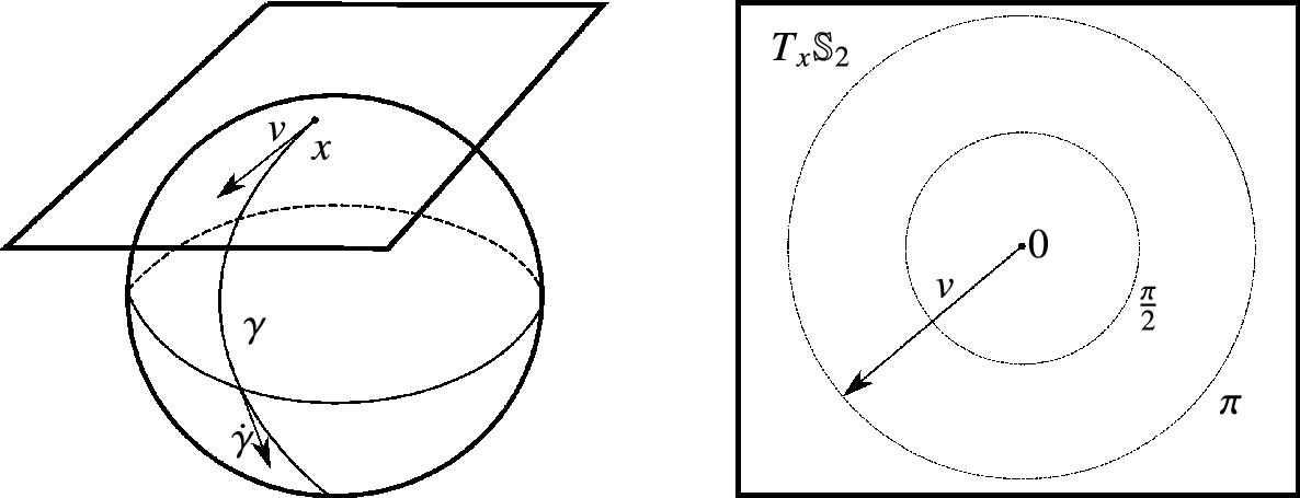
The map F is said to give an implicit representation of the manifold. In the previous example, we used the definition with F(x)=(x1)2+(x2)2+(x3)2−1![]() (see Fig. 1.1).
(see Fig. 1.1).

 of the map F:Rk→Rm
 . Here F:R3→R
 is given by the sphere equation x↦(x1)2+(x2)2+(x3)2−1
 , and the manifold M=S2
 is of dimension 3 − 1 = 2.
The fact that M=F−1(0)![]() is a manifold is often taken as the consequence of the submersion level set theorem instead of a definition. The theorem states that with the above assumptions, M
is a manifold is often taken as the consequence of the submersion level set theorem instead of a definition. The theorem states that with the above assumptions, M![]() has a manifold structure as constructed with charts and atlases. In addition, the topological and differentiable structure of M is in a certain way compatible with that of Rk
has a manifold structure as constructed with charts and atlases. In addition, the topological and differentiable structure of M is in a certain way compatible with that of Rk![]() letting us denote M as embedded in Rk
letting us denote M as embedded in Rk![]() . For now, we will be somewhat relaxed about the details and use the construction as a working definition of what we think of as a manifold.
. For now, we will be somewhat relaxed about the details and use the construction as a working definition of what we think of as a manifold.
The map F can be seen as a set of m constraints that points in M![]() must satisfy. The Jacobian matrix dF(x)
must satisfy. The Jacobian matrix dF(x)![]() at a point in x∈M
at a point in x∈M![]() linearizes the constraints around x, and its rank k−d
linearizes the constraints around x, and its rank k−d![]() indicates how many of them are linearly independent. In addition to the unit length constraints of vectors in R3
indicates how many of them are linearly independent. In addition to the unit length constraints of vectors in R3![]() defining S2
defining S2![]() , additional examples of commonly occurring manifolds that we will see in this book arise directly from embedded manifolds or as quotients of embedded manifolds.
, additional examples of commonly occurring manifolds that we will see in this book arise directly from embedded manifolds or as quotients of embedded manifolds.
Example 1.1
d-dimensional spheres Sd![]() embedded in Rd+1
embedded in Rd+1![]() . Here we express the unit length equation generalizing (1.1) by
. Here we express the unit length equation generalizing (1.1) by
Sd={x∈Rn+1|‖x‖2−1=0}.
The squared norm ‖x‖2![]() is the standard squared Euclidean norm on Rd+1
is the standard squared Euclidean norm on Rd+1![]() .
.
Example 1.2
Orthogonal matrices O(k)![]() on Rk
on Rk![]() have the property that the inner products 〈Ui,Uj〉
have the property that the inner products 〈Ui,Uj〉![]() of columns Ui
of columns Ui![]() , Uj
, Uj![]() of the matrix U∈M(k,k)
of the matrix U∈M(k,k)![]() vanish for i≠j
vanish for i≠j![]() and equal 1 for i=j
and equal 1 for i=j![]() . This gives k2
. This gives k2![]() constraints, and O(k)
constraints, and O(k)![]() is thus an embedded manifold in M(k,k)
is thus an embedded manifold in M(k,k)![]() by the equation
by the equation
O(k)={U∈M(k,k)|UU⊤−Idk=0}
with Idk![]() being the identity matrix on Rk
being the identity matrix on Rk![]() . We will see in Section 1.7.3 that the rank of the map F(U)=UU⊤−Idk
. We will see in Section 1.7.3 that the rank of the map F(U)=UU⊤−Idk![]() is k(k+1)2
is k(k+1)2![]() on O(k)
on O(k)![]() , and it follows that O(k)
, and it follows that O(k)![]() has dimension k(k−1)2
has dimension k(k−1)2![]() .
.
1.2.2 Charts and local euclideaness
We now describe how charts, local parameterizations of the manifold, can be constructed from the implicit representation above. We will use this to give a more abstract definition of a differentiable manifold.
When navigating the surface of the earth, we seldom use curved representations of the surface but instead rely on charts that give a flat, 2D representation of regions limited in extent. It turns out that this analogy can be extended to embed manifolds with a rigorous mathematical formulation.
Definition 1.2
A chart on a d-dimensional manifold M![]() is a diffeomorphic mapping ϕ:U→˜U
is a diffeomorphic mapping ϕ:U→˜U![]() from an open set U⊂M
from an open set U⊂M![]() to an open set ˜U⊆Rd
to an open set ˜U⊆Rd![]() .
.
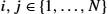
The definition exactly captures the informal idea of representing a local part of the surface, the open set U, with a mapping to a Euclidean space, in the surface case R2![]() (see Fig. 1.2).
(see Fig. 1.2).
 and ψ:V→˜V
 , members of the atlas covering the manifold M
 , from the open sets U,V⊂M
 to open sets ˜U
 , ˜V
, ˜V of Rd
of Rd , respectively. The compatibility condition ensures that ϕ and ψ agree on the overlap U ∩ V between U and V in the sense that the composition ψ∘ϕ−1 is a differentiable map.
When using charts, we often say that we work in coordinates. Instead of accessing points on M![]() directly, we take a chart ϕ:U→˜U
directly, we take a chart ϕ:U→˜U![]() and use points in ϕ(U)⊆Rd
and use points in ϕ(U)⊆Rd![]() instead. This gives us the convenience of having a coordinate system present. However, we need to be aware that the choice of the coordinate system affects the analysis, both theoretically and computationally. When we say that we work in coordinates x=(x1,…,xd)
instead. This gives us the convenience of having a coordinate system present. However, we need to be aware that the choice of the coordinate system affects the analysis, both theoretically and computationally. When we say that we work in coordinates x=(x1,…,xd)![]() , we implicitly imply that there is a chart ϕ such that ϕ−1(x)
, we implicitly imply that there is a chart ϕ such that ϕ−1(x)![]() is a point on M
is a point on M![]() .
.
It is a consequence of the implicit function theorem that embedded manifolds have charts. Proving it takes some work, but we can sketch the idea in the case of the implicit representation map F:Rk→Rm![]() having Jacobian with full rank m. Recall the setting of the implicit function theorem (see e.g. [18]): Let F:Rd+m→Rm
having Jacobian with full rank m. Recall the setting of the implicit function theorem (see e.g. [18]): Let F:Rd+m→Rm![]() be continuously differentiable and write (x,y)∈Rd+m
be continuously differentiable and write (x,y)∈Rd+m![]() such that x denotes the first d coordinates and y the last m coordinates. Let dyF
such that x denotes the first d coordinates and y the last m coordinates. Let dyF![]() denote the last m columns of the Jacobian matrix dF, that is, the derivatives of F taken with respect to variations in y. If dyF
denote the last m columns of the Jacobian matrix dF, that is, the derivatives of F taken with respect to variations in y. If dyF![]() has full rank m at a point (x,y)
has full rank m at a point (x,y)![]() where F(x,y)=0
where F(x,y)=0![]() , then there exists an open neighborhood ˜U⊆Rd
, then there exists an open neighborhood ˜U⊆Rd![]() of x and a differentiable map g:˜U→Rm
of x and a differentiable map g:˜U→Rm![]() such that F(x,g(x))=0
such that F(x,g(x))=0![]() for all x∈˜U
for all x∈˜U![]() .
.
The only obstruction to using the implicit function theorem directly to find charts is that we may need to rotate the coordinates on Rd+m![]() to find coordinates (x,y)
to find coordinates (x,y)![]() and a submatrix dyF
and a submatrix dyF![]() of full rank. With this in mind, the map g ensures that F(x,g(x))=0
of full rank. With this in mind, the map g ensures that F(x,g(x))=0![]() for all x∈˜U
for all x∈˜U![]() , that is, the points (x,g(x)),x∈˜U
, that is, the points (x,g(x)),x∈˜U![]() are included in M
are included in M![]() . Setting U=g(˜U)
. Setting U=g(˜U)![]() , we get a chart ϕ:U→˜U
, we get a chart ϕ:U→˜U![]() directly by the mapping (x,g(x))↦x
directly by the mapping (x,g(x))↦x![]() .
.
1.2.3 Abstract manifolds and atlases
We now use the concept of charts to define atlases as collections of charts and from this the abstract notion of a manifold.
Definition 1.3
Atlas
An atlas of a set M![]() is a family of charts (ϕi)i=1,…,N
is a family of charts (ϕi)i=1,…,N![]() , ϕi:Ui→˜Ui
, ϕi:Ui→˜Ui![]() such that
such that
- • ϕi
 cover M: For each x∈M
 , there exists i∈{1,…,N}
 such that x∈Ui
 ,
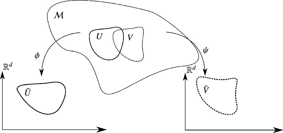
, - • ϕi are compatible: For each pair i,j∈{1,…,N}
 where Ui∩Uj
 is nonempty, the composition ϕi∘ϕ−1j:ϕj(Ui∩Uj)→Rd
 is a differentiable map.
An atlas thus ensures the existence of at least one chart covering a neighborhood of each point of M![]() . This allows the topological and differential structure of M
. This allows the topological and differential structure of M![]() to be given by a definition from the topology and differential structure of the image of the charts, that is, Rd
to be given by a definition from the topology and differential structure of the image of the charts, that is, Rd![]() . Intuitively, the structure coming from the Euclidean spaces Rd
. Intuitively, the structure coming from the Euclidean spaces Rd![]() is pulled back using ϕi
is pulled back using ϕi![]() to the manifold. In order for this construction to work, we must ensure that there is no ambiguity in the structure we get if the domain of multiple charts cover a given point. The compatibility condition ensures exactly that.
to the manifold. In order for this construction to work, we must ensure that there is no ambiguity in the structure we get if the domain of multiple charts cover a given point. The compatibility condition ensures exactly that.
Definition 1.4
Manifold
Let M![]() be a set with an atlas (ϕi)i=1,…,N
be a set with an atlas (ϕi)i=1,…,N![]() with ϕi:Ui→˜Ui
with ϕi:Ui→˜Ui![]() , ˜Ui⊆Rd
, ˜Ui⊆Rd![]() . Then M
. Then M![]() is a manifold of dimension d.
is a manifold of dimension d.
Remark 1.1
Until now, we have been somewhat loose in describing maps as being “differentiable”. The differentiability of maps on a manifold comes from the differential structure, which in turn is defined from the atlas and the charts mapping to Rd![]() . The differential structure on Rd
. The differential structure on Rd![]() allows derivatives up to any order, but the charts may not support this when transferring the structure to M
allows derivatives up to any order, but the charts may not support this when transferring the structure to M![]() . To be more precise, in the compatibility condition, we require the compositions ϕi∘ϕ−1j
. To be more precise, in the compatibility condition, we require the compositions ϕi∘ϕ−1j![]() to be Cr
to be Cr![]() as maps from Rd
as maps from Rd![]() to Rd
to Rd![]() for some integer r. This gives a differentiable structure on M
for some integer r. This gives a differentiable structure on M![]() of the same order. In particular, when r≥1
of the same order. In particular, when r≥1![]() , we say that M
, we say that M![]() is a differentiable manifold, and M
is a differentiable manifold, and M![]() is smooth if r=∞
is smooth if r=∞![]() . We may also require only r=0
. We may also require only r=0![]() , in which case M
, in which case M![]() is a topological manifold with no differentiable structure.
is a topological manifold with no differentiable structure.
Because of the implicit function theorem, embedded submanifolds in the sense of Definition 1.1 have charts and atlases. Embedded submanifolds are therefore particular examples of abstract manifolds. In fact, this goes both ways: The Whitney embedding theorem states that any d-dimensional manifold can be embedded in Rk![]() with k⩽2d
with k⩽2d![]() so that the topology is induced by the one of the embedding space. For Riemannian manifolds defined later on, this theorem only provides a local C1
so that the topology is induced by the one of the embedding space. For Riemannian manifolds defined later on, this theorem only provides a local C1![]() embedding and not a global smooth embedding.
embedding and not a global smooth embedding.
Example 1.3
The projective space Pd![]() is the set of lines through the origin in Rd+1
is the set of lines through the origin in Rd+1![]() . Each such line intersects the sphere Sd
. Each such line intersects the sphere Sd![]() in two points that are antipodal. By identifying such points, expressed by taking the quotient using the equivalence relation x∼−x
in two points that are antipodal. By identifying such points, expressed by taking the quotient using the equivalence relation x∼−x![]() , we get the representation Pd≃Sd/∼
, we get the representation Pd≃Sd/∼![]() . Depending on the properties of the equivalence relation, the quotient space of a manifold may not be a manifold in general (more details will be given in Chapter 9). In the case of the projective space, we can verify the above abstract manifold definition. Therefore the projective space cannot be seen as an embedded manifold directly, but it can be seen as the quotient space of an embedded manifold.
. Depending on the properties of the equivalence relation, the quotient space of a manifold may not be a manifold in general (more details will be given in Chapter 9). In the case of the projective space, we can verify the above abstract manifold definition. Therefore the projective space cannot be seen as an embedded manifold directly, but it can be seen as the quotient space of an embedded manifold.
1.2.4 Tangent vectors and tangent space
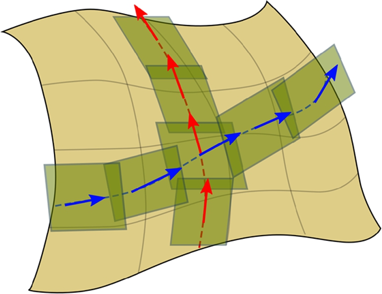
As the name implies, derivatives lies at the core of differential geometry. The differentiable structure allows taking derivatives of curves in much the same way as the usual derivatives in Euclidean space. However, spaces of tangent vectors to curves behave somewhat differently on manifolds due to the lack of the global reference frame that the Euclidean space coordinate system gives. We here discuss derivatives of curves, tangent vectors, and tangent spaces.
Let γ:[0,T]→Rk![]() be a differentiable curve in Rk
be a differentiable curve in Rk![]() parameterized on the interval [0,T]
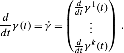
parameterized on the interval [0,T]![]() . For each t, the curve derivative is
. For each t, the curve derivative is
ddtγ(t)=˙γ=(ddtγ1(t)⋮ddtγk(t)).
This tangent or velocity vector can be regarded as a vector in Rk![]() , denoted the tangent vector to γ at t. If M
, denoted the tangent vector to γ at t. If M![]() is an embedded manifold in Rk
is an embedded manifold in Rk![]() and γ(t)∈M
and γ(t)∈M![]() for all t∈[0,T]
for all t∈[0,T]![]() , we can regard γ as a curve in M
, we can regard γ as a curve in M![]() . As illustrated on Fig. 1.3, the tangent vectors of γ are also tangential to M
. As illustrated on Fig. 1.3, the tangent vectors of γ are also tangential to M![]() itself. The set of tangent vectors to all curves at x=γ(t)
itself. The set of tangent vectors to all curves at x=γ(t)![]() span a d-dimensional affine subspace of Rk
span a d-dimensional affine subspace of Rk![]() that approximates M
that approximates M![]() to the first order at x. This affine space has an explicit realization as x+kerdF(x)
to the first order at x. This affine space has an explicit realization as x+kerdF(x)![]() where x=γ(t)
where x=γ(t)![]() is the foot-point and kerdF
is the foot-point and kerdF![]() denotes the kernel (null-space) of the Jacobian matrix of F. The space is called the tangent space TxM
denotes the kernel (null-space) of the Jacobian matrix of F. The space is called the tangent space TxM![]() of M
of M![]() at the point x. In the embedded manifold case, tangent vectors thus arise from the standard curve derivative, and tangent spaces are affine subspaces of Rk
at the point x. In the embedded manifold case, tangent vectors thus arise from the standard curve derivative, and tangent spaces are affine subspaces of Rk![]() .
.
 . If M is embedded, then γ is in addition a curve in Rk
 . The derivative ˙γ(t)
 is a tangent vector in the linear tangent space Tγ(t)M
 . It can be written in coordinates using ϕ as ˙γ=˙γi∂xi
 . In the embedding space, the tangent space Tγ(t)M is the affine d-dimensional subspace γ(t)+kerdF(γ(t))
 of Rk.
On abstract manifolds, the definition of tangent vectors becomes somewhat more intricate. Let γ be a curve in the abstract manifold M![]() , and consider t∈[0,T]
, and consider t∈[0,T]![]() . By the covering assumption on the atlas, there exists a chart ϕ:U→˜U
. By the covering assumption on the atlas, there exists a chart ϕ:U→˜U![]() with γ(t)∈U
with γ(t)∈U![]() . By the continuity of γ and openness of U, γ(s)∈U
. By the continuity of γ and openness of U, γ(s)∈U![]() for s sufficiently close to t. Now the curve ˜γ=ϕ∘γ
for s sufficiently close to t. Now the curve ˜γ=ϕ∘γ![]() in Rd
in Rd![]() is defined for such s. Thus we can take the standard Euclidean derivative ˙˜γ
is defined for such s. Thus we can take the standard Euclidean derivative ˙˜γ![]() of ˜γ
of ˜γ![]() . This gives a vector in Rd
. This gives a vector in Rd![]() . In the same way as we define the differentiable structure on M
. In the same way as we define the differentiable structure on M![]() by definition to be that inherited from the charts, it would be natural to let a tangent vector of M
by definition to be that inherited from the charts, it would be natural to let a tangent vector of M![]() be ˙˜γ
be ˙˜γ![]() by definition. However, we would like to be able to define tangent vectors independently of the underlying curve. In addition, we need to ensure that the construction does not depend on the chart ϕ.
by definition. However, we would like to be able to define tangent vectors independently of the underlying curve. In addition, we need to ensure that the construction does not depend on the chart ϕ.
One approach is to define tangent vectors from their actions on real-valued functions on M![]() . Let f:M→R
. Let f:M→R![]() be a differentiable function. Then f∘γ
be a differentiable function. Then f∘γ![]() is a function from R
is a function from R![]() to R
to R![]() whose derivative is
whose derivative is
ddtf∘γ(t).
This operation is clearly linear in f in the sense that ddt((αf+βg)∘γ)=αddt(f∘γ)+βddt(g∘γ)![]() when g is another differentiable function and α,β∈R
when g is another differentiable function and α,β∈R![]() . In addition, this derivative satisfies the usual product rule for the derivative of the pointwise product f⋅g
. In addition, this derivative satisfies the usual product rule for the derivative of the pointwise product f⋅g![]() of f and g. Operators on differentiable functions satisfying these properties are called derivations, and we can define tangent vectors and tangent spaces as the set of derivations, that is, v∈TxM
of f and g. Operators on differentiable functions satisfying these properties are called derivations, and we can define tangent vectors and tangent spaces as the set of derivations, that is, v∈TxM![]() is a tangent vector if it defines a derivation v(f)
is a tangent vector if it defines a derivation v(f)![]() on functions f∈C1(M,R)
on functions f∈C1(M,R)![]() . It can now be checked that the curve derivative using a chart above defines derivations. By the chain rule we can see that these derivations are independent of the chosen chart.
. It can now be checked that the curve derivative using a chart above defines derivations. By the chain rule we can see that these derivations are independent of the chosen chart.
The construction of TxM![]() as derivations is rather abstract. In practice, it is often most convenient to just remember that there is an abstract definition and otherwise think of tangent vectors as derivatives of curves. In fact, tangent vectors and tangent spaces can also be defined without derivations using only the derivatives of curves. However, in this case, we must define a tangent vector as an equivalence class of curves because multiple curves can result in the same derivative. This construction, although in some sense more intuitive, therefore has its own complexities.
as derivations is rather abstract. In practice, it is often most convenient to just remember that there is an abstract definition and otherwise think of tangent vectors as derivatives of curves. In fact, tangent vectors and tangent spaces can also be defined without derivations using only the derivatives of curves. However, in this case, we must define a tangent vector as an equivalence class of curves because multiple curves can result in the same derivative. This construction, although in some sense more intuitive, therefore has its own complexities.
The set {TxM|x∈M}![]() has a structure of a differentiable manifold in itself. It is called the tangent bundle TM
has a structure of a differentiable manifold in itself. It is called the tangent bundle TM![]() . It follows that tangent vectors v∈TxM
. It follows that tangent vectors v∈TxM![]() for some x∈M
for some x∈M![]() are elements of TM
are elements of TM![]() . TM
. TM![]() is a particular case of a fiber bundle (a local product of spaces whose global topology may be more complex). We will later see other examples of fiber bundles, for example, the cotangent bundle T⁎M
is a particular case of a fiber bundle (a local product of spaces whose global topology may be more complex). We will later see other examples of fiber bundles, for example, the cotangent bundle T⁎M![]() and the frame bundle FM
and the frame bundle FM![]() .
.
A local coordinate system x=(x1,…xd)![]() coming from a chart induces a basis ∂x=(∂x1,…∂xd)
coming from a chart induces a basis ∂x=(∂x1,…∂xd)![]() of the tangent space TxM
of the tangent space TxM![]() . Therefore any v∈TxM
. Therefore any v∈TxM![]() can be expressed as a linear combination of ∂x1,…∂xd
can be expressed as a linear combination of ∂x1,…∂xd![]() . Writing vi
. Writing vi![]() for the ith entry of such linear combinations, we have v=∑di=1vi∂xi
for the ith entry of such linear combinations, we have v=∑di=1vi∂xi![]() .
.
Remark 1.2
Einstein summation convention
We will often use the Einstein summation convention that dictates an implicit sum over indices appearing twice in lower and upper position in expressions, in particular, in coordinate expressions and tensor calculations. For example, in the coordinate basis mentioned above, we have v=vi∂xi![]() , where the sum ∑di=1
, where the sum ∑di=1![]() is implicit because the index i appears in upper position on vi
is implicit because the index i appears in upper position on vi![]() and lower position on ∂xi
and lower position on ∂xi![]() .
.
Just as a Euclidean vector space V has a dual vector space V⁎![]() consisting of linear functionals ξ:V→R
consisting of linear functionals ξ:V→R![]() , the tangent spaces TxM
, the tangent spaces TxM![]() and tangent bundle TM
and tangent bundle TM![]() have dual spaces, the cotangent spaces T⁎xM
have dual spaces, the cotangent spaces T⁎xM![]() , and cotangent bundle T⁎M
, and cotangent bundle T⁎M![]() . For each x, elements of the cotangent space T⁎xM
. For each x, elements of the cotangent space T⁎xM![]() are linear maps from TxM
are linear maps from TxM![]() to R
to R![]() . The coordinate basis (∂x1,…∂xd)
. The coordinate basis (∂x1,…∂xd)![]() induces a similar coordinate basis (dx1,…dxd)
induces a similar coordinate basis (dx1,…dxd)![]() for the cotangent space. This basis is defined from evaluation on ∂xi
for the cotangent space. This basis is defined from evaluation on ∂xi![]() by dxj(∂xi)=δji
by dxj(∂xi)=δji![]() , where the delta-function δji
, where the delta-function δji![]() is 1 if i=j
is 1 if i=j![]() and 0 otherwise. The coordinates vi
and 0 otherwise. The coordinates vi![]() for tangent vectors in the coordinate basis had upper indices above. Similarly, coordinates for cotangent vectors conventionally have lower indices such that ξ=ξidxi
for tangent vectors in the coordinate basis had upper indices above. Similarly, coordinates for cotangent vectors conventionally have lower indices such that ξ=ξidxi![]() for ξ∈T⁎xM
for ξ∈T⁎xM![]() again using the Einstein summation convention. Elements of T⁎M
again using the Einstein summation convention. Elements of T⁎M![]() are called covectors. The evaluation ξ(v)
are called covectors. The evaluation ξ(v)![]() of a covector ξ on a vector v is sometimes written (ξ|v)
of a covector ξ on a vector v is sometimes written (ξ|v)![]() or 〈ξ,v〉
or 〈ξ,v〉![]() . Note that the latter notation with brackets is similar to the notation for inner products used later on.
. Note that the latter notation with brackets is similar to the notation for inner products used later on.
1.2.5 Differentials and pushforward
The interpretation of tangent vectors as derivations allows taking derivatives of functions. If X is a vector field on M![]() , then we can use this pointwise to define a new function on M
, then we can use this pointwise to define a new function on M![]() by taking derivatives at each point, that is, X(f)(x)=X(x)(f)
by taking derivatives at each point, that is, X(f)(x)=X(x)(f)![]() using that X(x)
using that X(x)![]() is a tangent vector in TxM
is a tangent vector in TxM![]() and hence a derivation that acts on functions. If instead f is a map between two manifolds f:M→N
and hence a derivation that acts on functions. If instead f is a map between two manifolds f:M→N![]() , then we get the differential df:TM→TN
, then we get the differential df:TM→TN![]() as a map between the tangent bundle of M
as a map between the tangent bundle of M![]() and N
and N![]() . In coordinates, this is df(∂xi)j=∂xifj
. In coordinates, this is df(∂xi)j=∂xifj![]() with fj
with fj![]() being the jth component of f. The differential df is often denoted the pushforward of f because it uses f to map, that is, push, tangent vectors in TM
being the jth component of f. The differential df is often denoted the pushforward of f because it uses f to map, that is, push, tangent vectors in TM![]() to tangent vectors in TN
to tangent vectors in TN![]() . For this reason, the pushforward notation f⁎=df
. For this reason, the pushforward notation f⁎=df![]() is often used. When f is invertible, there exists a corresponding pullback operation f⁎=df−1
is often used. When f is invertible, there exists a corresponding pullback operation f⁎=df−1![]() .
.
As a particular case, consider a map f between M![]() and the manifold R
and the manifold R![]() . Then f⁎=df
. Then f⁎=df![]() is a map from TM
is a map from TM![]() to TR
to TR![]() . Because R
. Because R![]() is Euclidean, we can identify the tangent bundle with R
is Euclidean, we can identify the tangent bundle with R![]() itself, and we can consider df a map TM→R
itself, and we can consider df a map TM→R![]() . Being a derivative, df|TxM
. Being a derivative, df|TxM![]() is linear for each x∈M
is linear for each x∈M![]() , and df(x)
, and df(x)![]() is therefore a covector in T⁎xM
is therefore a covector in T⁎xM![]() . Though the differential df is also a pushforward, the notation df is most often used because of its interpretation as a covector field.
. Though the differential df is also a pushforward, the notation df is most often used because of its interpretation as a covector field.
1.3 Riemannian manifolds
So far, we defined manifolds as having topological and differential structure, either inherited from Rk![]() when considering embedded manifolds, or via charts and atlases with the abstract definition of manifolds. We now start including geometric and metric structures.
when considering embedded manifolds, or via charts and atlases with the abstract definition of manifolds. We now start including geometric and metric structures.
The topology determines the local structure of a manifold by specifying the open sets and thereby continuity of curves and functions. The differentiable structure allowed us to define tangent vectors and differentiate functions on the manifold. However, we have not yet defined a notion of how “straight” manifold-valued curves are. To obtain such a notion, we need to add a geometric structure, called a connection, which allows us to compare neighboring tangent spaces and characterizes the parallelism of vectors at different points. Indeed, differentiating a curve on a manifold gives tangent vectors belonging at each point to a different tangent vector space. To compute the second-order derivative, the acceleration of the curves, we need a way to map the tangent space at a point to the tangent space at any neighboring point. This is the role of a connection ∇XY![]() , which specifies how the vector field Y(x)
, which specifies how the vector field Y(x)![]() is derived in the direction of the vector field X(x)
is derived in the direction of the vector field X(x)![]() (Fig. 1.4). In the embedding case, tangent spaces are affine spaces of the embedding vector space, and the simplest way to specify this mapping is through an affine transformation, hence the name affine connection introduced by Cartan [3]. A connection operator also describes how a vector is transported from a tangent space to a neighboring one along a given curve. Integrating this transport along the curve specifies the parallel transport along this curve. However, there is usually no global parallelism as in Euclidean space. As a matter of fact, transporting the same vector along two different curves arriving at the same point in general leads to different vectors at the endpoint. This is easily seen on the sphere when traveling from north pole to the equator, then along the equator for 90 degrees and back to north pole turns any tangent vector by 90 degrees. This defect of global parallelism is the sign of curvature.
(Fig. 1.4). In the embedding case, tangent spaces are affine spaces of the embedding vector space, and the simplest way to specify this mapping is through an affine transformation, hence the name affine connection introduced by Cartan [3]. A connection operator also describes how a vector is transported from a tangent space to a neighboring one along a given curve. Integrating this transport along the curve specifies the parallel transport along this curve. However, there is usually no global parallelism as in Euclidean space. As a matter of fact, transporting the same vector along two different curves arriving at the same point in general leads to different vectors at the endpoint. This is easily seen on the sphere when traveling from north pole to the equator, then along the equator for 90 degrees and back to north pole turns any tangent vector by 90 degrees. This defect of global parallelism is the sign of curvature.
By looking for curves that remain locally parallel to themselves, that is, such that ∇˙γ˙γ=0![]() , we define the equivalent of “straight lines” in the manifold, geodesics. We should notice that there exists many different choices of connections on a given manifold, which lead to different geodesics. However, geodesics by themselves do not quantify how far away from each other two points are. For that purpose, we need an additional structure, a distance. By restricting to distances that are compatible with the differential structure, we enter into the realm of Riemannian geometry.
, we define the equivalent of “straight lines” in the manifold, geodesics. We should notice that there exists many different choices of connections on a given manifold, which lead to different geodesics. However, geodesics by themselves do not quantify how far away from each other two points are. For that purpose, we need an additional structure, a distance. By restricting to distances that are compatible with the differential structure, we enter into the realm of Riemannian geometry.
1.3.1 Riemannian metric
A Riemannian metric is defined by a smoothly varying collection of scalar products 〈⋅,⋅〉x![]() on each tangent space TxM
on each tangent space TxM![]() at points x of the manifold. For each x, each such scalar product is a positive definite bilinear map 〈⋅,⋅〉x:TxM×TxM→R
at points x of the manifold. For each x, each such scalar product is a positive definite bilinear map 〈⋅,⋅〉x:TxM×TxM→R![]() ; see Fig. 1.5. The inner product gives a norm ‖⋅‖x:TxM→R
; see Fig. 1.5. The inner product gives a norm ‖⋅‖x:TxM→R![]() by ‖v‖2=〈v,v〉x
by ‖v‖2=〈v,v〉x![]() . In a given chart we can express the metric by a symmetric positive definite matrix g(x)
. In a given chart we can express the metric by a symmetric positive definite matrix g(x)![]() . The ijth entry of the matrix is denoted gij(x)
. The ijth entry of the matrix is denoted gij(x)![]() and given by the dot product of the coordinate basis for the tangent space, gij(x)=〈∂xi,∂xj〉x
and given by the dot product of the coordinate basis for the tangent space, gij(x)=〈∂xi,∂xj〉x![]() . This matrix is called the local representation of the Riemannian metric in the chart x, and the dot product of two vectors v and w in TxM
. This matrix is called the local representation of the Riemannian metric in the chart x, and the dot product of two vectors v and w in TxM![]() is now in coordinates 〈v,w〉x=v⊤g(x)w=vigij(x)wj
is now in coordinates 〈v,w〉x=v⊤g(x)w=vigij(x)wj![]() . The components gij
. The components gij![]() of the inverse g(x)−1
of the inverse g(x)−1![]() of the metric defines a metric on covectors by 〈ξ,η〉x=ξigijηj
of the metric defines a metric on covectors by 〈ξ,η〉x=ξigijηj![]() . Notice how the upper indices of gij
. Notice how the upper indices of gij![]() fit the lower indices of the covector in the Einstein summation convention. This inner product on T⁎xM
fit the lower indices of the covector in the Einstein summation convention. This inner product on T⁎xM![]() is called a cometric.
is called a cometric.

 along the curve γ live in different tangent spaces and therefore cannot be compared directly. A connection ∇ defines a notion of transport of vectors along curves. This allows transport of a vector ˙γ(t−Δt)∈Tγ(t−Δt)M
 to Tγ(t)M, and the acceleration ∇˙γ˙γ
 arises by taking derivatives in Tγ(t)M. (Right) For each point x∈M, the metric g defines a positive bilinear map gx:TxM×TxM→R
 . Contrary to the Euclidean case, g depends on the base point, and vectors in the tangent space TyM
 can only be compared by g evaluated at y, that is, the map gy:TyM×TyM→R
 .
.1.3.2 Curve length and Riemannian distance
If we consider a curve γ(t)![]() on the manifold, then we can compute at each t its velocity vector ˙γ(t)
on the manifold, then we can compute at each t its velocity vector ˙γ(t)![]() and its norm ‖˙γ(t)‖
and its norm ‖˙γ(t)‖![]() , the instantaneous speed. For the velocity vector, we only need the differential structure, but for the norm, we need the Riemannian metric at the point γ(t)
, the instantaneous speed. For the velocity vector, we only need the differential structure, but for the norm, we need the Riemannian metric at the point γ(t)![]() . To compute the length of the curve, the norm is integrated along the curve:
. To compute the length of the curve, the norm is integrated along the curve:
L(γ)=∫‖˙γ(t)‖γ(t)dt=∫(〈˙γ(t),˙γ(t)〉γ(t))12dt.
The integrals here are over the domain of the curve, for example, [0,T]![]() . We write Lba(γ)=∫ba‖˙γ(t)‖γ(t)dt
. We write Lba(γ)=∫ba‖˙γ(t)‖γ(t)dt![]() to be explicit about the integration domain. This gives the length of the curve segment from γ(a)
to be explicit about the integration domain. This gives the length of the curve segment from γ(a)![]() to γ(b)
to γ(b)![]() .
.
The distance between two points of a connected Riemannian manifold is the minimum length among the curves γ joining these points:
dist(x,y)=minγ(0)=x,γ(1)=yL(γ).
The topology induced by this Riemannian distance is the original topology of the manifold: open balls constitute a basis of open sets.
The Riemannian metric is the intrinsic way of measuring length on a manifold. The extrinsic way is to consider the manifold as embedded in Rk![]() and compute the length of a curve in M
and compute the length of a curve in M![]() as for any curve in Rk
as for any curve in Rk![]() . In section 1.2.4 we identified the tangent spaces of an embedded manifold with affine subspaces of Rk
. In section 1.2.4 we identified the tangent spaces of an embedded manifold with affine subspaces of Rk![]() . In this case the Riemannian metric is the restriction of the dot product on Rk
. In this case the Riemannian metric is the restriction of the dot product on Rk![]() to the tangent space at each point of the manifold. Embedded manifolds thus inherit also their geometric structure in the form of the Riemannian metric from the embedding space.
to the tangent space at each point of the manifold. Embedded manifolds thus inherit also their geometric structure in the form of the Riemannian metric from the embedding space.
1.3.3 Geodesics
In Riemannian manifolds, locally length-minimizing curves are called metric geodesics. The next subsection will show that these curves are also autoparallel for a specific connection, so that they are simply called geodesics in general. A curve is locally length minimizing if for all t and sufficiently small s, Lt+st(γ)=dist(γ(t),γ(t+s))![]() . This implies that small segments of the curve realize the Riemannian distance. Finding such curves is complicated by the fact that any time-reparameterization of the curve is authorized. Thus geodesics are often defined as critical points of the energy functional E(γ)=12∫‖˙γ‖2dt
. This implies that small segments of the curve realize the Riemannian distance. Finding such curves is complicated by the fact that any time-reparameterization of the curve is authorized. Thus geodesics are often defined as critical points of the energy functional E(γ)=12∫‖˙γ‖2dt![]() . It turns out that critical points for the energy also optimize the length functional. Moreover, they are parameterized proportionally to their arc length removing the ambiguity of the parameterization.
. It turns out that critical points for the energy also optimize the length functional. Moreover, they are parameterized proportionally to their arc length removing the ambiguity of the parameterization.
We now define the Christoffel symbols from the metric g by
Γkij=12gkm(∂xigjm+∂xjgmi−∂xmgij).
Using the calculus of variations, it can be shown that the geodesics satisfy the second-order differential system
¨γk+Γkij˙γi˙γj=0.
We will see the Christoffel symbols again in coordinate expressions for the connection below.
1.3.4 Levi-Civita connection
The fundamental theorem of Riemannian geometry states that on any Riemannian manifold, there is a unique connection which is compatible with the metric and which has the property of being torsion-free. This connection is called the Levi-Civita connection. For that choice of connection, shortest curves have zero acceleration and are thus geodesics in the sense of being “straight lines”. In the following we only consider the Levi-Civita connection unless explicitly stated.
The connection allows us to take derivatives of a vector field Y in the direction of another vector field X expressed as ∇XY![]() . This is also denoted the covariant derivative of Y along X. The connection is linear in X and obeys the product rule in Y so that ∇X(fY)=X(f)Y+f∇XY
. This is also denoted the covariant derivative of Y along X. The connection is linear in X and obeys the product rule in Y so that ∇X(fY)=X(f)Y+f∇XY![]() for a function f:M→R
for a function f:M→R![]() with X(f)
with X(f)![]() being the derivative of f in the direction of X using the interpretation of tangent vectors as derivations. In a local coordinate system we can write the connection explicitly using the Christoffel symbols by ∇∂xi∂xj=Γkij∂xk
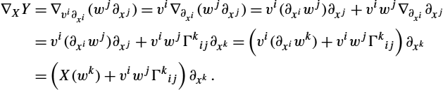
being the derivative of f in the direction of X using the interpretation of tangent vectors as derivations. In a local coordinate system we can write the connection explicitly using the Christoffel symbols by ∇∂xi∂xj=Γkij∂xk![]() . With vector fields X and Y having coordinates X(x)=vi(x)∂xi
. With vector fields X and Y having coordinates X(x)=vi(x)∂xi![]() and Y(x)=wi(x)∂xi
and Y(x)=wi(x)∂xi![]() , we can use this to compute the coordinate expression for derivatives of Y along X:
, we can use this to compute the coordinate expression for derivatives of Y along X:
∇XY=∇vi∂xi(wj∂xj)=vi∇∂xi(wj∂xj)=vi(∂xiwj)∂xj+viwj∇∂xi∂xj=vi(∂xiwj)∂xj+viwjΓkij∂xk=(vi(∂xiwk)+viwjΓkij)∂xk=(X(wk)+viwjΓkij)∂xk.
Using this, the connection allows us to write the geodesic equation (1.8) as the zero acceleration constraint:
0=∇˙γ˙γ=(˙γ(˙γk)+˙γi˙γjΓkij)∂xk=(¨γk+˙γi˙γjΓkij)∂xk.
The connection also defines the notion of parallel transport along curves. A vector v∈Tγ(t0)M![]() is parallel transported if it is extended to a t-dependent family of vectors with v(t)∈Tγ(t)M
is parallel transported if it is extended to a t-dependent family of vectors with v(t)∈Tγ(t)M![]() and ∇˙γ(t)v(t)=0
and ∇˙γ(t)v(t)=0![]() for each t. Parallel transport can thereby be seen as a map Pγ,t:Tγ(t0)M→Tγ(t)M
for each t. Parallel transport can thereby be seen as a map Pγ,t:Tγ(t0)M→Tγ(t)M![]() linking tangent spaces. The parallel transport inherits linearity from the connection. It follows from the definition that γ is a geodesic precisely if ˙γ(t)=Pγ,t(˙γ(t0))
linking tangent spaces. The parallel transport inherits linearity from the connection. It follows from the definition that γ is a geodesic precisely if ˙γ(t)=Pγ,t(˙γ(t0))![]() .
.
It is a fundamental consequence of curvature that parallel transport depends on the curve along which the vector is transported: With curvature, the parallel transports Pγ,T![]() and Pϕ,T
and Pϕ,T![]() along two curves γ and ϕ with the same end-points γ(t0)=ϕ(t0)
along two curves γ and ϕ with the same end-points γ(t0)=ϕ(t0)![]() and γ(T)=ϕ(T)
and γ(T)=ϕ(T)![]() will differ. The difference is denoted holonomy, and the holonomy of a Riemannian manifold vanishes only if M
will differ. The difference is denoted holonomy, and the holonomy of a Riemannian manifold vanishes only if M![]() is flat, that is, has zero curvature.
is flat, that is, has zero curvature.
1.3.5 Completeness
The Riemannian manifold is said to be geodesically complete if the definition domain of all geodesics can be extended to R![]() . This means that the manifold has neither boundary nor any singular point that we can reach in a finite time. For instance, Rd−{0}
. This means that the manifold has neither boundary nor any singular point that we can reach in a finite time. For instance, Rd−{0}![]() with the usual metric is not geodesically complete because some geodesics will hit 0 and thus stop being defined in finite time. On the other hand, Rd
with the usual metric is not geodesically complete because some geodesics will hit 0 and thus stop being defined in finite time. On the other hand, Rd![]() is geodesically complete. Other examples of complete Riemannian manifolds include compact manifolds implying that Sd
is geodesically complete. Other examples of complete Riemannian manifolds include compact manifolds implying that Sd![]() is geodesically complete. This is a consequence of the Hopf–Rinow–de Rham theorem, which also states that geodesically complete manifolds are complete metric spaces with the induced distance and that there always exists at least one minimizing geodesic between any two points of the manifold, that is, a curve whose length is the distance between the two points.
is geodesically complete. This is a consequence of the Hopf–Rinow–de Rham theorem, which also states that geodesically complete manifolds are complete metric spaces with the induced distance and that there always exists at least one minimizing geodesic between any two points of the manifold, that is, a curve whose length is the distance between the two points.
From now on, we will assume that the manifold is geodesically complete. This assumption is one of the fundamental properties ensuring the well-posedness of algorithms for computing on manifolds.
1.3.6 Exponential and logarithm maps
Let x be a point of the manifold that we consider as a local reference point, and let v be a vector of the tangent space TxM![]() at that point. From the theory of second-order differential equations, it can be shown that there exists a unique geodesic γ(x,v)(t)
at that point. From the theory of second-order differential equations, it can be shown that there exists a unique geodesic γ(x,v)(t)![]() starting from that point x=γ(x,v)(0)
starting from that point x=γ(x,v)(0)![]() with tangent vector v=˙γ(x,v)(0)
with tangent vector v=˙γ(x,v)(0)![]() . This geodesic is first defined in a sufficiently small interval around zero, but since the manifold is assumed geodesically complete, its definition domain can be extended to R
. This geodesic is first defined in a sufficiently small interval around zero, but since the manifold is assumed geodesically complete, its definition domain can be extended to R![]() . Thus the points γ(x,v)(t)
. Thus the points γ(x,v)(t)![]() are defined for each t and each v∈TxM
are defined for each t and each v∈TxM![]() . This allows us to map vectors in the tangent space to the manifold using geodesics: the vector v∈TxM
. This allows us to map vectors in the tangent space to the manifold using geodesics: the vector v∈TxM![]() can be mapped to the point of the manifold that is reached after a unit time t=1
can be mapped to the point of the manifold that is reached after a unit time t=1![]() by the geodesic γ(x,v)(t)
by the geodesic γ(x,v)(t)![]() starting at x with tangent vector v. This mapping
starting at x with tangent vector v. This mapping
Expx:TxM⟶Mv⟼Expx(v)=γ(x,v)(1)
is called the exponential map at point x. Straight lines passing 0 in the tangent space are transformed into geodesics passing the point x on the manifold, and the distances along these lines are conserved (Fig. 1.6).
 are images of the exponential map γ(t)=Expx(tv). They have zero acceleration ∇˙γ˙γ, and their velocity vectors are parallel transported ˙γ(t)=Pγ,t(˙γ(t0))
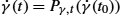 . Geodesics locally realize the Riemannian distance so that dist(x,γ(t))=t‖v‖
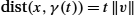 for sufficiently small t. (Right) The tangent space TxS2
 and Expx give an exponential chart mapping vectors v∈TxS2
 to points in S2
 by Expx(v). The cut locus of x is its antipodal point, and the injectivity radius is π. Note that the equator is the set {Expx(v)|‖v‖=π2}
 .
.When the manifold is geodesically complete, the exponential map is defined on the entire tangent space TxM![]() , but it is generally one-to-one only locally around 0 in the tangent space corresponding to a local neighborhood of x on M
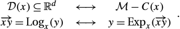
, but it is generally one-to-one only locally around 0 in the tangent space corresponding to a local neighborhood of x on M![]() . We denote by →xy
. We denote by →xy![]() or Logx(y)
or Logx(y)![]() the inverse of the exponential map where the inverse is defined: this is the smallest vector as measured by the Riemannian metric such that y=Expx(→xy)
the inverse of the exponential map where the inverse is defined: this is the smallest vector as measured by the Riemannian metric such that y=Expx(→xy)![]() . In this chart the geodesics going through x are represented by the lines going through the origin: Logxγ(x,→xy)(t)=t→xy
. In this chart the geodesics going through x are represented by the lines going through the origin: Logxγ(x,→xy)(t)=t→xy![]() . Moreover, the distance with respect to the base point x is preserved:
. Moreover, the distance with respect to the base point x is preserved:
dist(x,y)=‖→xy‖=√〈→xy,→xy〉x.
Thus the exponential chart at x gives a local representation of the manifold in the tangent space at a given point. This is also called a normal coordinate system or normal chart if it is provided with an orthonormal basis. At the origin of such a chart, the metric reduces to the identity matrix, and the Christoffel symbols vanish. Note again that the exponential map is generally only invertible locally around 0∈TxM![]() , and Logxy
, and Logxy![]() is therefore only locally defined, that is, for points y near x.
is therefore only locally defined, that is, for points y near x.
The exponential and logarithm maps are commonly referred to as the Exp and Log maps.
1.3.7 Cut locus
It is natural to search for the maximal domain where the exponential map is a diffeomorphism. If we follow a geodesic γ(x,v)(t)=Expx(tv)![]() from t=0
from t=0![]() to infinity, then it is either always minimizing for all t, or it is minimizing up to a time t0<∞
to infinity, then it is either always minimizing for all t, or it is minimizing up to a time t0<∞![]() . In this last case the point z=γ(x,v)(t0)
. In this last case the point z=γ(x,v)(t0)![]() is called a cut point, and the corresponding tangent vector t0v
is called a cut point, and the corresponding tangent vector t0v![]() is called a tangential cut point. The set of all cut points of all geodesics starting from x is the cut locus C(x)∈M
is called a tangential cut point. The set of all cut points of all geodesics starting from x is the cut locus C(x)∈M![]() , and the set of corresponding vectors is the tangential cut locus C(x)∈TxM
, and the set of corresponding vectors is the tangential cut locus C(x)∈TxM![]() . Thus we have C(x)=Expx(C(x))
. Thus we have C(x)=Expx(C(x))![]() , and the maximal definition domain for the exponential chart is the domain
, and the maximal definition domain for the exponential chart is the domain ![]() containing 0 and delimited by the tangential cut locus.
containing 0 and delimited by the tangential cut locus.
It is easy to see that this domain is connected and star-shaped with respect to the origin of ![]() . Its image by the exponential map covers the manifold except the cut locus, and the segment
. Its image by the exponential map covers the manifold except the cut locus, and the segment ![]() is transformed into the unique minimizing geodesic from x to y. Hence, the exponential chart has a connected and star-shaped definition domain that covers all the manifold except the cut locus
is transformed into the unique minimizing geodesic from x to y. Hence, the exponential chart has a connected and star-shaped definition domain that covers all the manifold except the cut locus ![]() :
:
From a computational point of view, it is often interesting to extend this representation to include the tangential cut locus. However, we have to take care of the multiple representations: Points in the cut locus where several minimizing geodesics meet are represented by several points on the tangential cut locus as the geodesics are starting with different tangent vectors (e.g. antipodal points on the sphere and rotation of π around a given axis for 3D rotations). This multiplicity problem cannot be avoided as the set of such points is dense in the cut locus.
The size of ![]() is quantified by the injectivity radius
is quantified by the injectivity radius ![]() , which is the maximal radius of centered balls in
, which is the maximal radius of centered balls in ![]() on which the exponential map is one-to-one. The injectivity radius of the manifold
on which the exponential map is one-to-one. The injectivity radius of the manifold ![]() is the infimum of the injectivity over the manifold. It may be zero, in which case the manifold somehow tends toward a singularity (e.g. think of the surface
is the infimum of the injectivity over the manifold. It may be zero, in which case the manifold somehow tends toward a singularity (e.g. think of the surface ![]() as a submanifold of
as a submanifold of ![]() ).
).
Example 1.4
On the sphere ![]() (center 0 and radius 1) with the canonical Riemannian metric (induced by the ambient Euclidean space
(center 0 and radius 1) with the canonical Riemannian metric (induced by the ambient Euclidean space ![]() ), the geodesics are the great circles, and the cut locus of a point x is its antipodal point
), the geodesics are the great circles, and the cut locus of a point x is its antipodal point ![]() . The exponential chart is obtained by rolling the sphere onto its tangent space so that the great circles going through p become lines. The maximal definition domain is thus the open ball
. The exponential chart is obtained by rolling the sphere onto its tangent space so that the great circles going through p become lines. The maximal definition domain is thus the open ball ![]() . On its boundary
. On its boundary ![]() , all the points represent
, all the points represent ![]() ; see Fig. 1.6.
; see Fig. 1.6.
For the real projective space ![]() (obtained by identification of antipodal points of the sphere
(obtained by identification of antipodal points of the sphere ![]() ), the geodesics are still the great circles, but the cut locus of the point
), the geodesics are still the great circles, but the cut locus of the point ![]() is now the equator of the two points, with antipodal points identified (thus the cut locus is
is now the equator of the two points, with antipodal points identified (thus the cut locus is ![]() ). The definition domain of the exponential chart is the open ball
). The definition domain of the exponential chart is the open ball ![]() , and the tangential cut locus is the sphere
, and the tangential cut locus is the sphere ![]() where antipodal points are identified.
where antipodal points are identified.
1.4 Elements of analysis in Riemannian manifolds
We here outline further constructions on manifolds relating to taking derivatives of functions, the intrinsic Riemannian measure, and defining curvature. These notions will be used in the following chapters of this book, for instance, for optimization algorithms.
1.4.1 Gradient and musical isomorphisms
Let f be a smooth function from ![]() to
to ![]() . Recall that the differential
. Recall that the differential ![]() evaluated at the point
evaluated at the point ![]() is a covector in
is a covector in ![]() . Therefore, contrary to the Euclidean situation where derivatives are often regarded as vectors, we cannot directly interpret
. Therefore, contrary to the Euclidean situation where derivatives are often regarded as vectors, we cannot directly interpret ![]() as a vector. However, thanks to the Riemannian metric, there is a canonical way to identify the linear form
as a vector. However, thanks to the Riemannian metric, there is a canonical way to identify the linear form ![]() with a unique vector
with a unique vector ![]() . This is done by defining
. This is done by defining ![]() to be a vector satisfying
to be a vector satisfying ![]() for all vectors
for all vectors ![]() . This mapping corresponds to the transpose operator that is implicitly used in Euclidean spaces to transform derivatives of functions (row vectors) to column vectors. On manifolds, the Riemannian metric must be specified explicitly since the coordinate system used may not be orthonormal everywhere.
. This mapping corresponds to the transpose operator that is implicitly used in Euclidean spaces to transform derivatives of functions (row vectors) to column vectors. On manifolds, the Riemannian metric must be specified explicitly since the coordinate system used may not be orthonormal everywhere.
The mapping works for any covector and is often denoted the sharp map ![]() . It has an inverse in the flat map
. It has an inverse in the flat map ![]() . In coordinates,
. In coordinates, ![]() for a covector
for a covector ![]() , and
, and ![]() for a vector
for a vector ![]() . The maps
. The maps ![]() and
and ![]() are denoted musical isomorphisms because they raise or lower the indices of the coordinates.
are denoted musical isomorphisms because they raise or lower the indices of the coordinates.
We can use the sharp map to define the Riemannian gradient as a vector:
This definition corresponds to the classical gradient in ![]() using the standard Euclidean inner product as a Riemannian metric. Using the coordinate representation of the sharp map, we get the coordinate form
using the standard Euclidean inner product as a Riemannian metric. Using the coordinate representation of the sharp map, we get the coordinate form ![]() of the gradient.
of the gradient.
1.4.2 Hessian and Taylor expansion
The covariant derivative of the gradient, the Hessian, arises from the connection ∇:
Here the two expressions on the right are given using the action of the connection on the differential form df (a covector) or the vector field ![]() . Its expression in a local coordinate system is
. Its expression in a local coordinate system is
Let now ![]() be the expression of f in a normal coordinate system at x. Its Taylor expansion around the origin in coordinates is
be the expression of f in a normal coordinate system at x. Its Taylor expansion around the origin in coordinates is
where ![]() is the Jacobian matrix of first-order derivatives, and
is the Jacobian matrix of first-order derivatives, and ![]() is the Euclidean Hessian matrix. Because the coordinate system is normal, we have
is the Euclidean Hessian matrix. Because the coordinate system is normal, we have ![]() . Moreover, the metric at the origin reduces to the identity:
. Moreover, the metric at the origin reduces to the identity: ![]() , and the Christoffel symbols vanish so that the matrix of second derivatives
, and the Christoffel symbols vanish so that the matrix of second derivatives ![]() corresponds to the Hessian Hess f. Thus the Taylor expansion can be written in any coordinate system:
corresponds to the Hessian Hess f. Thus the Taylor expansion can be written in any coordinate system:
1.4.3 Riemannian measure or volume form
In a vector space with basis ![]() the local representation of the metric is given by
the local representation of the metric is given by ![]() , where
, where ![]() is the matrix of coordinates change from
is the matrix of coordinates change from ![]() to an orthonormal basis. Similarly, the measure or the infinitesimal volume element is given by the volume of the parallelepiped spanned by the basis vectors:
to an orthonormal basis. Similarly, the measure or the infinitesimal volume element is given by the volume of the parallelepiped spanned by the basis vectors: ![]() with
with ![]() denoting the matrix determinant. In a Riemannian manifold
denoting the matrix determinant. In a Riemannian manifold ![]() , the Riemannian metric
, the Riemannian metric ![]() induces an infinitesimal volume element on each tangent space, and thus a measure on the manifold that in coordinates has the expression
induces an infinitesimal volume element on each tangent space, and thus a measure on the manifold that in coordinates has the expression
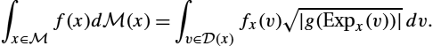
The cut locus has null measure, and we can therefore integrate indifferently in ![]() or in any exponential chart. If f is an integrable function of the manifold and
or in any exponential chart. If f is an integrable function of the manifold and ![]() is its image in the exponential chart at x, then we have
is its image in the exponential chart at x, then we have
1.4.4 Curvature
The curvature of a Riemannian manifold measures its deviance from local flatness. We often have a intuitive notion of when a surface embedded in ![]() is flat or curved; for example, a linear subspace of
is flat or curved; for example, a linear subspace of ![]() is flat, whereas the sphere
is flat, whereas the sphere ![]() is curved. This idea of curvature is expressed in the Gauss curvature. However, for high-dimensional spaces, the mathematical description becomes somewhat more intricate. We will further on see several notions of curvature capturing aspects of the nonlinearity of the manifold with varying details. It is important to note that whereas vanishing curvature implies local flatness of the manifold, this is not the same as the manifold being globally Euclidean. An example is the torus
is curved. This idea of curvature is expressed in the Gauss curvature. However, for high-dimensional spaces, the mathematical description becomes somewhat more intricate. We will further on see several notions of curvature capturing aspects of the nonlinearity of the manifold with varying details. It is important to note that whereas vanishing curvature implies local flatness of the manifold, this is not the same as the manifold being globally Euclidean. An example is the torus ![]() , which can both be embedded in
, which can both be embedded in ![]() inheriting nonzero curvature and be embedded in
inheriting nonzero curvature and be embedded in ![]() in a way in which it inherits a flat geometry. In both cases the periodicity of the torus remains, which prevents it from being a vector space.
in a way in which it inherits a flat geometry. In both cases the periodicity of the torus remains, which prevents it from being a vector space.
The curvature of a Riemannian manifold is described by the curvature tensor ![]() . It is defined from the covariant derivative by evaluation on vector fields X, Y, Z:
. It is defined from the covariant derivative by evaluation on vector fields X, Y, Z:
The bracket ![]() denotes the anticommutativity of the fields X and Y. If f is a differentiable function on
denotes the anticommutativity of the fields X and Y. If f is a differentiable function on ![]() , then the new vector field produced by the bracket is given by its application to f:
, then the new vector field produced by the bracket is given by its application to f: ![]() . The curvature tensor R can intuitively be interpreted at
. The curvature tensor R can intuitively be interpreted at ![]() as the difference between parallel transporting the vector
as the difference between parallel transporting the vector ![]() along an infinitesimal parallelogram with sides
along an infinitesimal parallelogram with sides ![]() and
and ![]() ; see Fig. 1.7 (left). As noted earlier, parallel transport is curve dependent, and the difference between transporting infinitesimally along
; see Fig. 1.7 (left). As noted earlier, parallel transport is curve dependent, and the difference between transporting infinitesimally along ![]() and then
and then ![]() as opposed to along
as opposed to along ![]() and then
and then ![]() is a vector in
is a vector in ![]() . This difference can be calculated for any vector
. This difference can be calculated for any vector ![]() . The curvature tensor when evaluated at X, Y, that is,
. The curvature tensor when evaluated at X, Y, that is, ![]() , is the linear map
, is the linear map ![]() given by this difference.
given by this difference.

 . The principal curvatures arise from comparing these geodesics to circles as for the Euclidean notion of curvature of a curve.
The reader should note that two different sign conventions exist for the curvature tensor: definition (1.10) is used in a number of reference books in physics and mathematics [20,16,14,24,11]. Other authors use a minus sign to simplify some of the tensor notations [26,21,4,5,1] and different order conventions for the tensors subscripts and/or a minus sign in the sectional curvature defined below (see e.g. the discussion in [6, p. 399]).
The curvature can be realized in coordinates from the Christoffel symbols:

The sectional curvature κ measures the Gaussian curvature of 2D submanifolds of ![]() , the Gaussian curvature of each point being the product of the principal curvatures of curves passing the point. The 2D manifolds arise as the geodesic spray of a 2D linear subspace of
, the Gaussian curvature of each point being the product of the principal curvatures of curves passing the point. The 2D manifolds arise as the geodesic spray of a 2D linear subspace of ![]() ; see Fig. 1.7 (right). Such a 2-plane can be represented by basis vectors
; see Fig. 1.7 (right). Such a 2-plane can be represented by basis vectors ![]() , in which case the sectional curvature can be expressed using the curvature tensor by
, in which case the sectional curvature can be expressed using the curvature tensor by
The curvature tensor gives the notion of Ricci and scalar curvatures, which both provide summary information of the full tensor R. The Ricci curvature Ric is the trace over the first and last indices of R with coordinate expression
Taking another trace, we get the scalar valued quantity, the scalar curvature S:
Note that the cometric appears to raise one index before taking the trace.
1.5 Lie groups and homogeneous manifolds
A Lie group is a manifold equipped with additional group structure such that the group multiplication and group inverse are smooth mappings. Many of the interesting transformations used in image analysis, translations, rotations, affine transforms, and so on, form Lie groups. We will in addition see examples of infinite-dimensional Lie groups when doing shape analysis with diffeomorphisms as described in chapter 4. We begin by reviewing the definition of an algebraic group.
Definition 1.5
Group
A group is a set G with a binary operation, denoted here by concatenation or group product, such that
- 1.
 for all
  ,
, - 2. there is an identity element
 satisfying
  for all
  ,
, - 3. each has an inverse
 satisfying
  .
.
A Lie group is simultaneously a group and a manifold, with compatibility between these two mathematical concepts.
Definition 1.6
Lie Group

Example 1.5
The space of all ![]() nonsingular matrices forms a Lie group called the general linear group, denoted
nonsingular matrices forms a Lie group called the general linear group, denoted ![]() . The group operation is matrix multiplication, and
. The group operation is matrix multiplication, and ![]() can be given a smooth manifold structure as an open subset of
can be given a smooth manifold structure as an open subset of ![]() . The equations for matrix multiplication and inverse are smooth operations in the entries of the matrices. Thus
. The equations for matrix multiplication and inverse are smooth operations in the entries of the matrices. Thus ![]() satisfies the requirements of a Lie group in Definition 1.6. A matrix group is any closed subgroup of
satisfies the requirements of a Lie group in Definition 1.6. A matrix group is any closed subgroup of ![]() . Matrix groups inherit the smooth structure of
. Matrix groups inherit the smooth structure of ![]() as a subset of
as a subset of ![]() and are thus also Lie groups.
and are thus also Lie groups.
Example 1.6
The ![]() rotation matrices form a closed matrix subgroup of
rotation matrices form a closed matrix subgroup of ![]() and thus a Lie group. This group is called the special orthogonal group. It is defined as
and thus a Lie group. This group is called the special orthogonal group. It is defined as ![]() . This space is a closed bounded subset of
. This space is a closed bounded subset of ![]() and thus compact.
and thus compact.
For each y in a Lie group G, the following two diffeomorphisms of G are denoted left- and right-translations by y:

The differential or pushforward ![]() of the left translation maps the tangent space
of the left translation maps the tangent space ![]() to the tangent space
to the tangent space ![]() . In particular,
. In particular, ![]() maps any vector
maps any vector ![]() to the vector
to the vector ![]() thereby giving rise to the vector field
thereby giving rise to the vector field ![]() . Such a vector field is said to be left-invariant since it is invariant under left multiplication:
. Such a vector field is said to be left-invariant since it is invariant under left multiplication: ![]() for every
for every ![]() . Right-invariant vector fields are defined similarly. A left- or right-invariant vector field is uniquely defined by its value
. Right-invariant vector fields are defined similarly. A left- or right-invariant vector field is uniquely defined by its value ![]() on the tangent space at the identity.
on the tangent space at the identity.
Recall that vector fields on G can be seen as derivations on the space of smooth functions ![]() . Thus two vector fields u and v can be composed to form another operator uv on
. Thus two vector fields u and v can be composed to form another operator uv on ![]() , but the operator uv is not necessarily a derivation as it includes second-order differential terms. However, the operator
, but the operator uv is not necessarily a derivation as it includes second-order differential terms. However, the operator ![]() is a vector field on G. Indeed, we can check by writing this expression in a local coordinate system that the second-order terms vanish. This leads to a definition of the Lie bracket of vector fields u, v on G, defined as
is a vector field on G. Indeed, we can check by writing this expression in a local coordinate system that the second-order terms vanish. This leads to a definition of the Lie bracket of vector fields u, v on G, defined as
This is also sometimes called the Lie derivative ![]() because it is conceptually the derivative of the vector field v in the direction
because it is conceptually the derivative of the vector field v in the direction ![]() generated by u at each point
generated by u at each point ![]() .
.
Definition 1.7
Lie algebra
A Lie algebra is a vector space V equipped with a bilinear product ![]() , called a Lie bracket, that satisfies
, called a Lie bracket, that satisfies
- 1.
 (skew symmetry) for all
  ,
, - 2.
 (Jacobi identity) for all
  .
.
The tangent space ![]() of a Lie group G at the identity element, typically denoted
of a Lie group G at the identity element, typically denoted ![]() , forms a Lie algebra. The Lie bracket on
, forms a Lie algebra. The Lie bracket on ![]() is induced by the Lie bracket on the corresponding left-invariant vector fields. For two vectors u, v in
is induced by the Lie bracket on the corresponding left-invariant vector fields. For two vectors u, v in ![]() , let
, let ![]() ,
, ![]() be the corresponding unique left-invariant vector fields on G. Then the Lie bracket on
be the corresponding unique left-invariant vector fields on G. Then the Lie bracket on ![]() is given by
is given by
The Lie bracket provides a test for whether the Lie group G is commutative. A Lie group G is commutative if and only if the Lie bracket on the corresponding Lie algebra ![]() is zero, that is,
is zero, that is, ![]() for all
for all ![]() .
.
Example 1.8
The Lie algebra for Euclidean space ![]() is again
is again ![]() . The Lie bracket is zero, that is,
. The Lie bracket is zero, that is, ![]() for all
for all ![]() .
.
Example 1.9
The Lie algebra for ![]() is
is ![]() , the space of all real
, the space of all real ![]() matrices. The Lie bracket operation for
matrices. The Lie bracket operation for ![]() is given by
is given by
Here the product XY denotes actual matrix multiplication, which turns out to be the same as composition of the vector field operators (compare to (1.15)). All Lie algebras corresponding to matrix groups are subalgebras of ![]() .
.
Example 1.10
The Lie algebra for the rotation group ![]() is
is ![]() , the space of skew-symmetric matrices. A matrix A is skew-symmetric if
, the space of skew-symmetric matrices. A matrix A is skew-symmetric if ![]() .
.
Let is called a one-parameter subgroup because it is a morphing of Lie groups: Let Definition 1.8 Action A left action of a Lie group G on a manifold We will see examples of Lie group actions throughout the book. For example, Chapter 4 on shape analysis relies fundamentally on actions of the group Through the action, a curve in Some particularly important actions are the actions of G on itself and on the Lie algebra From the adjoint action, we get the adjoint operator The actions on the Lie algebra have dual actions as well, denoted coactions: the coadjoint action Let the group G act on The left- and right-translation maps give a particularly useful way of defining Riemannian metrics on Lie groups. Given an inner product This defines a left-invariant Riemannian metric on G because to get a right-invariant metric. In the particular case where the metric is invariant to both left- and right-translations, it is called biinvariant. Geodesics for biinvariant metrics are precisely one-parameter subgroups, and the Lie group exponential map exp therefore equals the Riemannian exponential map 1.5.1 One-parameter subgroups
![]() be a left-invariant vector field. The solution
be a left-invariant vector field. The solution ![]() to the initial value problem
to the initial value problem![]() . The Lie exponential map
. The Lie exponential map ![]() is then given by the value of
is then given by the value of ![]() at
at ![]() , that is,
, that is, ![]() . For matrix groups where the Lie group algebra consists of ordinary matrices, exp corresponds to the matrix exponential. The group exponential should not be confused with the Riemannian exponential as they usually differ, unless the group is provided with a biinvariant Riemannian metric.
. For matrix groups where the Lie group algebra consists of ordinary matrices, exp corresponds to the matrix exponential. The group exponential should not be confused with the Riemannian exponential as they usually differ, unless the group is provided with a biinvariant Riemannian metric.1.5.2 Actions
![]() be a manifold, and let G be a Lie group. The elements of the group can often be used to produce variations of elements of the manifold, for example, elements of
be a manifold, and let G be a Lie group. The elements of the group can often be used to produce variations of elements of the manifold, for example, elements of ![]() linearly transform elements of the manifold
linearly transform elements of the manifold ![]() . Similarly, affine transformations apply to change images in image registration. These are examples of actions of G on
. Similarly, affine transformations apply to change images in image registration. These are examples of actions of G on ![]() . Such actions are usually denoted
. Such actions are usually denoted ![]() where
where ![]() ,
, ![]() . Because the action involves two manifolds, G and
. Because the action involves two manifolds, G and ![]() , we will use x, y to denote elements of
, we will use x, y to denote elements of ![]() and g, h to denote elements of G.
and g, h to denote elements of G. ![]() is a smooth mapping
is a smooth mapping ![]() satisfying
satisfying![]() ,
, ![]() ,
,![]() ,
, ![]() ,
,![]() is a diffeomorphism of M for each
is a diffeomorphism of M for each ![]() .
.![]() of diffeomorphisms of a domain Ω on shape spaces
of diffeomorphisms of a domain Ω on shape spaces ![]() .
.![]() on the group G acts on a point
on the group G acts on a point ![]() to give a curve
to give a curve ![]() in
in ![]() . In particular, one-parameter subgroups define the curves
. In particular, one-parameter subgroups define the curves ![]() in
in ![]() for Lie algebra elements
for Lie algebra elements ![]() . The derivative
. The derivative![]() is denoted the infinitesimal generator associated with v.
is denoted the infinitesimal generator associated with v.![]() . These include the actions by left translation
. These include the actions by left translation ![]() and the action by conjugation
and the action by conjugation ![]() . The pushforward of the conjugation gives the adjoint action
. The pushforward of the conjugation gives the adjoint action ![]() of G on
of G on ![]() . The adjoint action is also denoted
. The adjoint action is also denoted ![]() .
.![]() for
for ![]() . This operator is sometimes informally denoted “little ad”, and it is related to the Lie bracket by
. This operator is sometimes informally denoted “little ad”, and it is related to the Lie bracket by ![]() .
.![]() ,
, ![]() for
for ![]() , where the dual of the adjoint is given by
, where the dual of the adjoint is given by ![]() for all
for all ![]() . Using the notation
. Using the notation ![]() for evaluation
for evaluation ![]() of ξ on v, the definition of the dual of the adjoint is
of ξ on v, the definition of the dual of the adjoint is ![]() . The coadjoint operator
. The coadjoint operator ![]() is similarly specified by
is similarly specified by ![]() for
for ![]() and
and ![]() .
.1.5.3 Homogeneous spaces
![]() . If, for any
. If, for any ![]() , there exists
, there exists ![]() such that
such that ![]() , then the action is said to be transitive. In this case the manifold
, then the action is said to be transitive. In this case the manifold ![]() is homogeneous. For a fixed
is homogeneous. For a fixed ![]() , the closed subgroup
, the closed subgroup ![]() is denoted the isotropy subgroup of G, and
is denoted the isotropy subgroup of G, and ![]() is isomorphic to the quotient
is isomorphic to the quotient ![]() . Similarly, a closed subgroup H of G leads to a homogeneous space
. Similarly, a closed subgroup H of G leads to a homogeneous space ![]() by quotienting out H. Examples of homogeneous spaces are the spheres
by quotienting out H. Examples of homogeneous spaces are the spheres ![]() and the orbit shape spaces described in Chapter 4, for example, the manifold of landmark configurations.
and the orbit shape spaces described in Chapter 4, for example, the manifold of landmark configurations.1.5.4 Invariant metrics and geodesics
![]() on the Lie algebra, we can extend it to an inner product on tangent spaces at all elements of the group by setting
on the Lie algebra, we can extend it to an inner product on tangent spaces at all elements of the group by setting![]() for any
for any ![]() . Similarly, we can set
. Similarly, we can set![]() . For metrics that are left- or right-invariant, but not biinvariant, the ordinary geodesic equation (1.8) can be simplified using, for example, Euler–Poincaré reduction. The resulting Euler–Poincaré equations are discussed further in Chapter 4 in the case of right-invariant metrics on the group
. For metrics that are left- or right-invariant, but not biinvariant, the ordinary geodesic equation (1.8) can be simplified using, for example, Euler–Poincaré reduction. The resulting Euler–Poincaré equations are discussed further in Chapter 4 in the case of right-invariant metrics on the group ![]() .
.
1.6 Elements of computing on Riemannian manifolds
The Riemannian Exp and Log maps constitute very powerful atomic functions to express most geometric operations for performing statistical computing on manifolds. The implementation of ![]() and
and ![]() is therefore the algorithmic basis of programming on Riemannian manifolds, as we will further see.
is therefore the algorithmic basis of programming on Riemannian manifolds, as we will further see.
In a Euclidean space, exponential charts are nothing but orthonormal coordinates systems translated to each point: In this case ![]() and
and ![]() . This example is more than a simple coincidence. In fact, most of the usual operations using additions and subtractions may be reinterpreted in a Riemannian framework using the notion of bipoint, an antecedent of vector introduced during the 19th century. Indeed, vectors are defined as equivalent classes of bipoints, oriented couples of points, in a Euclidean space. This is possible using the canonical way to compare what happens at two different points by translating. In a Riemannian manifold we can compare vectors using the parallel transport along curves, but the curve dependence on the parallel transport prevents global comparison of vectors as in Euclidean space. This implies that each vector has to remember at which point of the manifold it is attached, as is the case for tangent vectors, which relates back to the Euclidean notion of a bipoint.
. This example is more than a simple coincidence. In fact, most of the usual operations using additions and subtractions may be reinterpreted in a Riemannian framework using the notion of bipoint, an antecedent of vector introduced during the 19th century. Indeed, vectors are defined as equivalent classes of bipoints, oriented couples of points, in a Euclidean space. This is possible using the canonical way to compare what happens at two different points by translating. In a Riemannian manifold we can compare vectors using the parallel transport along curves, but the curve dependence on the parallel transport prevents global comparison of vectors as in Euclidean space. This implies that each vector has to remember at which point of the manifold it is attached, as is the case for tangent vectors, which relates back to the Euclidean notion of a bipoint.
Conversely, the logarithm map may be used to map almost any bipoint ![]() into a vector
into a vector ![]() of
of ![]() . This reinterpretation of addition and subtraction using logarithm and exponential maps is very powerful when generalizing algorithms working on vector spaces to algorithms on Riemannian manifolds. This is illustrated in Table 1.1 and in the following sections.
. This reinterpretation of addition and subtraction using logarithm and exponential maps is very powerful when generalizing algorithms working on vector spaces to algorithms on Riemannian manifolds. This is illustrated in Table 1.1 and in the following sections.
Table 1.1
| Euclidean space | Riemannian manifold | |
|---|---|---|
| Subtraction | ||
| Addition | y = x + v | y = Expx(v) |
| Distance | dist(x,y)=‖y − x‖ | |
| Mean value (implicit) | ||
| Gradient descent | xt+ε = xt − ε∇f(xt) | |
| Geodesic interpolation |
The Exp and Log maps are different for each manifold and for each metric. They must therefore be determined and implemented on a case-by-case basis. In some cases, closed-form expressions are known, examples being the spheres ![]() , rotations and rigid body transformations with left-invariant metric [22], and covariance matrices (positive definite symmetric matrices, so-called tensors in medical image analysis) [23] and Chapter 3. In cases where closed-form solutions are not known, geodesics with given initial velocity can be obtained by numerically solving the geodesic ODE (1.8) or by solving the variational problem of finding a minimum energy curve between two points. Thus computing
, rotations and rigid body transformations with left-invariant metric [22], and covariance matrices (positive definite symmetric matrices, so-called tensors in medical image analysis) [23] and Chapter 3. In cases where closed-form solutions are not known, geodesics with given initial velocity can be obtained by numerically solving the geodesic ODE (1.8) or by solving the variational problem of finding a minimum energy curve between two points. Thus computing ![]() may be posed as a numerical integration problem (see e.g. [10,9]) and computing
may be posed as a numerical integration problem (see e.g. [10,9]) and computing ![]() as an optimal control problem. This opens the way to statistical computing in more complex spaces than the spaces we have considered up to now, such as spaces of curves, surfaces, and diffeomorphic transformations, as we will see in the following chapters. Geometric computation frameworks such as Theano Geometry1 [12] and Geomstats2 provide numerical implementations of geometric operations on some commonly used manifolds. Theano Geometry uses automatic differentiation to express and compute the derivatives that are essential for differential geometric computations. This results in a convenient code for computing Christoffel symbols, curvature tensors, and fiber bundle operations using the parallel transport.
as an optimal control problem. This opens the way to statistical computing in more complex spaces than the spaces we have considered up to now, such as spaces of curves, surfaces, and diffeomorphic transformations, as we will see in the following chapters. Geometric computation frameworks such as Theano Geometry1 [12] and Geomstats2 provide numerical implementations of geometric operations on some commonly used manifolds. Theano Geometry uses automatic differentiation to express and compute the derivatives that are essential for differential geometric computations. This results in a convenient code for computing Christoffel symbols, curvature tensors, and fiber bundle operations using the parallel transport.
1.7 Examples
We further survey ways to express the Exp and Log maps on selected manifolds, at the same time exemplifying how particular structure of the spaces can be used for computations.
1.7.1 The sphere
Let x be a point in ![]() . From the embedding of
. From the embedding of ![]() in
in ![]() , the tangent space
, the tangent space ![]() can be identified with the d-dimensional vector space of all vectors in
can be identified with the d-dimensional vector space of all vectors in ![]() orthogonal to x. The inner product between two tangent vectors is then equivalent to the usual Euclidean inner product. The exponential map is given by a 2D rotation of x by an angle given by the norm of the tangent, that is,
orthogonal to x. The inner product between two tangent vectors is then equivalent to the usual Euclidean inner product. The exponential map is given by a 2D rotation of x by an angle given by the norm of the tangent, that is,
The log map between two points x, y on the sphere can be computed by finding the initial velocity of the rotation between the two points. Let ![]() denote the projection of the vector y onto x. Then
denote the projection of the vector y onto x. Then
1.7.2 2D Kendall shape space
The Kendall shape space [13] represents a shape as an equivalence class of all translations, rotations, and scalings of a set of k points, landmarks, in the plane. A configuration of k points in the 2D plane is considered a complex k-vector ![]() . Removing translation by requiring the centroid to be zero projects this point to the linear complex subspace
. Removing translation by requiring the centroid to be zero projects this point to the linear complex subspace ![]() , which is isomorphic to the space
, which is isomorphic to the space ![]() . Next, points in this subspace are deemed equivalent if they are a rotation and scaling of each other, which can be represented as multiplication by a complex number
. Next, points in this subspace are deemed equivalent if they are a rotation and scaling of each other, which can be represented as multiplication by a complex number ![]() , where ρ is the scaling factor, and θ is the rotation angle. The set of such equivalence classes forms the complex projective space
, where ρ is the scaling factor, and θ is the rotation angle. The set of such equivalence classes forms the complex projective space ![]() .
.
We think of a centered shape ![]() as representing the complex line
as representing the complex line ![]() , that is,
, that is, ![]() consists of all point configurations with the same shape as p. A tangent vector at
consists of all point configurations with the same shape as p. A tangent vector at ![]() is a complex vector
is a complex vector ![]() such that
such that ![]() . The exponential map is given by rotating the complex line
. The exponential map is given by rotating the complex line ![]() within V by the initial velocity v:
within V by the initial velocity v:
Likewise, the log map between two shapes ![]() is given by finding the initial velocity of the rotation between the two complex lines
is given by finding the initial velocity of the rotation between the two complex lines ![]() and
and ![]() . Let
. Let ![]() denote the projection of the vector q onto p. Then the log map is given by
denote the projection of the vector q onto p. Then the log map is given by

In Chapter 4 we will see an example of a different landmark space equipped with a geometric structure coming from the action of the diffeomorphism group.
1.7.3 Rotations
The set of orthogonal transformations ![]() on
on ![]() discussed in section 1.2.1 is the subset of linear maps of
discussed in section 1.2.1 is the subset of linear maps of ![]() , square matrices
, square matrices ![]() , that preserve the dot product:
, that preserve the dot product: ![]() . In particular, they conserve the norm of a vector:
. In particular, they conserve the norm of a vector: ![]() . This means that
. This means that ![]() for all vectors
for all vectors ![]() , which is possible if and only if the matrix U satisfies the quadratic constraint
, which is possible if and only if the matrix U satisfies the quadratic constraint ![]() . Thus the inverse transformation is
. Thus the inverse transformation is ![]() . The composition of two such maps obviously also preserves the dot product, so this forms the group of orthogonal transformations with the identity matrix
. The composition of two such maps obviously also preserves the dot product, so this forms the group of orthogonal transformations with the identity matrix ![]() as neutral element e:
as neutral element e:
Because the quadratic constraint is smooth and differentiable, ![]() constitute a Lie group, submanifold of the linear space of square matrices. However, it is not connected: Taking the determinant of the constraint gives
constitute a Lie group, submanifold of the linear space of square matrices. However, it is not connected: Taking the determinant of the constraint gives ![]() , so that
, so that ![]() . We see that there are two disconnected components of determinants +1 and −1 that cannot be joined by any continuous curve on the space of matrices. Such a curve would have to go through matrices with determinants between −1 and 1 since the determinant is a continuous function. The component of the negative determinant includes symmetries that reverse the orientation of the space. It is not a subgroup because the composition of two such transformations of a negative determinant has a positive determinant.
. We see that there are two disconnected components of determinants +1 and −1 that cannot be joined by any continuous curve on the space of matrices. Such a curve would have to go through matrices with determinants between −1 and 1 since the determinant is a continuous function. The component of the negative determinant includes symmetries that reverse the orientation of the space. It is not a subgroup because the composition of two such transformations of a negative determinant has a positive determinant.
The component of a positive determinant preserves the orientation of the space and is a subgroup, the group of rotations, or special orthogonal transformations:
Let ![]() be a curve drawn on
be a curve drawn on ![]() , considered as an embedded manifold in the vector space of matrices
, considered as an embedded manifold in the vector space of matrices ![]() . The constraint
. The constraint ![]() is differentiated into
is differentiated into
which means that ![]() and
and ![]() are skew-symmetric matrices. Thus the tangent space
are skew-symmetric matrices. Thus the tangent space ![]() at identity is the vector space of skew-symmetric matrices, and the tangent space at rotation
at identity is the vector space of skew-symmetric matrices, and the tangent space at rotation ![]() is its left or right translation:
is its left or right translation:
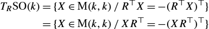
Since ![]() skew-symmetric matrices have
skew-symmetric matrices have ![]() free components, we also obtain that the dimension of the special orthogonal group is
free components, we also obtain that the dimension of the special orthogonal group is ![]() .
.
To put a metric on this Lie group, we may take a metric on the tangent space at the identity and left translate it to any other point resulting in a left-invariant metric. We may similarly right translate it to obtain a right-invariant metric. Since ![]() is a submanifold of the Euclidean space of matrices
is a submanifold of the Euclidean space of matrices ![]() , we may also consider the restriction of the embedding Frobenius dot product
, we may also consider the restriction of the embedding Frobenius dot product ![]() to the tangent spaces at all points. It is common to rescale the Frobenius metric by 1/2 to compensate the fact that we are counting twice each off diagonal coefficient of the skew-symmetric matrices. This induces the metric
to the tangent spaces at all points. It is common to rescale the Frobenius metric by 1/2 to compensate the fact that we are counting twice each off diagonal coefficient of the skew-symmetric matrices. This induces the metric
on the tangent space ![]() .
.
This metric is invariant by left and right translation. The existence of this biinvariant metric is a particular case due to the compactness of the ![]() group. Biinvariant metrics on Lie groups have very special properties, which will be described in Chapter 5. In particular, as mentioned earlier, geodesics passing the identity are one-parameter subgroups whose equations are given by the matrix exponential:
group. Biinvariant metrics on Lie groups have very special properties, which will be described in Chapter 5. In particular, as mentioned earlier, geodesics passing the identity are one-parameter subgroups whose equations are given by the matrix exponential: ![]() . This series is absolutely convergent, so that the matrix exponential always exists. Its inverse, the logarithm, may however fail to exist and is also generally not unique when it exists.
. This series is absolutely convergent, so that the matrix exponential always exists. Its inverse, the logarithm, may however fail to exist and is also generally not unique when it exists.
For rotations, the exponential of skew symmetric matrices covers the whole rotation group so that the log always exists, but it is not unique: For ![]() , rotating of an angle θ is the same as rotating of an angle
, rotating of an angle θ is the same as rotating of an angle ![]() , where l is an integer. To understand the structure of rotations in higher dimensions, we may look at the spectral decomposition of a rotation matrix R: The characteristic polynomial
, where l is an integer. To understand the structure of rotations in higher dimensions, we may look at the spectral decomposition of a rotation matrix R: The characteristic polynomial ![]() is a real polynomial of degree k. Thus the k complex eigenvalues are real or conjugate by pairs, and the polynomial can be factored into at most
is a real polynomial of degree k. Thus the k complex eigenvalues are real or conjugate by pairs, and the polynomial can be factored into at most ![]() quadratic terms, potentially with multiplicity, and real linear terms. The conservation of the norm by the rotation
quadratic terms, potentially with multiplicity, and real linear terms. The conservation of the norm by the rotation ![]() shows that the modulus of all the eigenvalues is 1. Thus eigenvalues are
shows that the modulus of all the eigenvalues is 1. Thus eigenvalues are ![]() or 1. Since a rotation is a normal matrix, it can be diagonalized, and we conclude that every rotation matrix, when expressed in a suitable coordinate system, partitions into
or 1. Since a rotation is a normal matrix, it can be diagonalized, and we conclude that every rotation matrix, when expressed in a suitable coordinate system, partitions into ![]() independent 2D rotations, called Givens rotations [8]:
independent 2D rotations, called Givens rotations [8]:

Conversely, each skew symmetric matrix ![]() decomposes the space
decomposes the space ![]() in a direct sum of mutually orthogonal subspaces, which are all invariant under Ω [8]. The decomposition has l (possibly equal to zero) two-dimensional vector subspaces
in a direct sum of mutually orthogonal subspaces, which are all invariant under Ω [8]. The decomposition has l (possibly equal to zero) two-dimensional vector subspaces ![]() on which Ω acts nontrivially, and one single subspace F of dimension
on which Ω acts nontrivially, and one single subspace F of dimension ![]() , the orthogonal complement of the span of other subspaces, which is the kernel of Ω. For any
, the orthogonal complement of the span of other subspaces, which is the kernel of Ω. For any ![]() , there exists an orthonormal basis of
, there exists an orthonormal basis of ![]() such that Ω restricted to
such that Ω restricted to ![]() is in this basis of the following matrix form:
is in this basis of the following matrix form: ![]() where
where ![]() (≠0) is the jth angle of rotation of the n-dimensional rotation
(≠0) is the jth angle of rotation of the n-dimensional rotation ![]() .
.
We can now come back to the uniqueness of the Log: When the angles of the above ![]() 2D rotations decomposing the rotation R are within
2D rotations decomposing the rotation R are within ![]() , the logarithm of R is well-defined. Otherwise, we cannot define a unique logarithm. This is only the case for 2D rotations of 180 degrees, whose two “smallest” real logarithms are
, the logarithm of R is well-defined. Otherwise, we cannot define a unique logarithm. This is only the case for 2D rotations of 180 degrees, whose two “smallest” real logarithms are ![]() and
and ![]() .
.
Geodesics starting at any point in the group are left, or right, translation of geodesics starting at identity. For instance, ![]() is the unique geodesic starting at R with tangent vector Y. The following reasoning underlies this: To find the geodesic starting at R with tangent vector Y, we first left translate Y by
is the unique geodesic starting at R with tangent vector Y. The following reasoning underlies this: To find the geodesic starting at R with tangent vector Y, we first left translate Y by ![]() to the tangent space at identity, compute the geodesic starting at e with tangent vector
to the tangent space at identity, compute the geodesic starting at e with tangent vector ![]() , and left translate back the result by R. Since the metric is biinvariant, the same mechanism can be implemented with right translation. The formula for the exponential map
, and left translate back the result by R. Since the metric is biinvariant, the same mechanism can be implemented with right translation. The formula for the exponential map ![]() at point R is thus
at point R is thus
Likewise, to compute the log map of rotation U at rotation R, we first left translate both rotations by ![]() , take the log map of
, take the log map of ![]() at e, and left translate back to result:
at e, and left translate back to result:
1.8 Additional references
This very compact introduction to differential geometry, Riemannian manifolds, and Lie groups provides only a brief overview of the underlying deep theory. We here provide some references to further reading. There are many excellent texts on the subjects. The following lists are therefore naturally nonexhaustive.
Introductory texts on differential and Riemannian geometry
- • J. M. Lee: Introduction to topological manifolds [17]; Introduction to smooth manifolds [18]; Riemannian manifolds [16].
- • M. do Carmo: Riemannian geometry [4].
- • J. Gallier: Notes on differential geometry manifolds, Lie groups and bundles, Chapter 3, http://www.cis.upenn.edu/~jean/gbooks/manif.html, [6].
- • S. Gallot, D. Hulin, J. Lafontaine; Riemannian geometry [5].
- • W. M. Boothby: An Introduction to differentiable manifolds and Riemannian geometry [2].
- • C. Small: Statistical theory of shapes [25].
Advanced differential and Riemannian geometry
- • J. Jost: Riemannian geometry and geometric analysis [11].
- • M. Berger: A panoramic view of Riemannian geometry [1].
- • I. Kolář, J. Slovák, P. W. M.: Natural operations in differential geometry [15].
- • P. W. Michor: Topics in differential geometry [19].
- • M. M. Postnikov: Geometry VI: Riemannian geometry [24].
Lie groups
- • S. Helgason: Differential geometry, Lie groups, and symmetric spaces [7].
- • J. Gallier: Notes on differential geometry manifolds, Lie groups and bundles, Chapters 2 and 4, http://www.cis.upenn.edu/~jean/gbooks/manif.html, [6].