
Chapter 2
Fractional Calculus and Fractional-Order Systems
2.1 Fractional Calculus
In this section, several important functions of fractional calculus, the definition of the fractional integral, three main fractional derivatives, and some important lemmas are introduced, which will be used throughout the book.
2.1.1 Several Important Functions of Fractional Calculus
In this subsection, three important functions of fractional calculus will be introduced: the gamma function, the beta function, and the Mittag–Leffler (ML) function.
On the basis of Equation (2.2), we have

2.1.2 Fractional Integral and Derivatives
In this subsection, we will introduce the definitions of the fractional integral and the three main fractional derivatives, i.e., the Grünwald–Letnikov (GL), Riemann–Liouville (RL), and Caputo definitions [154] [163–165].
In this definition, the initial time is set to zero. The same is true for the following definitions.
In this book, we use the definition of the Caputo fractional derivative to analyze the problems of control and synchronization control for fractional-order systems. Furthermore, we will use ![]() instead of
instead of ![]() .
.
2.1.3 Some Important Lemmas
In this subsection, some lemmas are introduced, which will be used to analyze the control for fractional-order systems in the book.
2.2 Some Typical Fractional-Order Systems
In this section, some fractional-order models are given; the dynamic behaviors of fractional-order systems are also shown by numerical simulation.
2.2.1 Fractional-Order Lorenz System
From the simplified equation of convective rolls in the equations of the atmosphere, the first three-dimensional chaotic system was derived by Lorenz in 1963 [178]. Furthermore, the developed fractional-order Lorenz system [179] is given as follows:

where ![]() ,
, ![]() , and
, and ![]() are fractional orders,
are fractional orders, ![]() ,
, ![]() , and
, and ![]() are system state variables, and
are system state variables, and ![]() ,
, ![]() , and
, and ![]() are system parameters. For fractional orders chosen as
are system parameters. For fractional orders chosen as ![]() , system parameters given by
, system parameters given by ![]() ,
, ![]() , and
, and ![]() , and initial conditions chosen as
, and initial conditions chosen as ![]() , the simulation results of the fractional-order Lorenz system are shown in Figure 2.1. Furthermore, the bifurcation diagram for
, the simulation results of the fractional-order Lorenz system are shown in Figure 2.1. Furthermore, the bifurcation diagram for ![]() is presented in Figure 2.2. Following the bifurcation diagram (Figure 2.2), the dynamic characteristic of two cycles for
is presented in Figure 2.2. Following the bifurcation diagram (Figure 2.2), the dynamic characteristic of two cycles for ![]() is shown in Figure 2.3.
is shown in Figure 2.3.

Figure 2.1 Chaotic behaviors of fractional-order Lorenz system (2.46): (a)  –
– plane; (b)
  –
– plane; (c)
  –
– plane; (d)
  –
– –
– space.

Figure 2.2 Bifurcation diagram of fractional-order Lorenz system (2.46) for  .
.

Figure 2.3 Dynamic characteristic of two cycles for fractional-order Lorenz system (2.46): (a)  –
– plane; (b)
  –
– plane; (c)
  –
– plane; (d)
  –
– –
– space.
2.2.2 Fractional-Order Van Der Pol Oscillator
The van der Pol oscillator is a non-conservative oscillator with nonlinear damping. The fractional-order van der Pol oscillator is given in the following form [164]:

where ![]() and
and ![]() are fractional orders,
are fractional orders, ![]() and
and ![]() are system state variables, and
are system state variables, and ![]() is a system parameter. For fractional orders chosen as
is a system parameter. For fractional orders chosen as ![]() and
and ![]() , the system parameter given by
, the system parameter given by ![]() , and initial conditions chosen as
, and initial conditions chosen as ![]() and
and ![]() , the simulation results of the fractional-order van der Pol oscillator are given in Figure 2.4.
, the simulation results of the fractional-order van der Pol oscillator are given in Figure 2.4.

Figure 2.4 Simulation result of fractional-order van der Pol oscillator (2.47).
2.2.3 Fractional-Order Genesio–Tesi System
The Genesio-Tesi system was first described using mathematical equations by Petrás̆ [164]. In addition, the fractional-order Genesio–Tesi system is defined as follows [180]:

where ![]() ,
, ![]() , and
, and ![]() are fractional orders,
are fractional orders, ![]() ,
, ![]() , and
, and ![]() are system state variables, and
are system state variables, and ![]() ,
, ![]() , and
, and ![]() are system parameters. For fractional orders chosen as
are system parameters. For fractional orders chosen as ![]() and
and ![]() , system parameters given by
, system parameters given by ![]() ,
, ![]() , and
, and ![]() , and initial conditions chosen as
, and initial conditions chosen as ![]() ,
, ![]() , and
, and ![]() , the simulation results of the fractional-order Genesio–Tesi system are presented in Figure 2.5. Furthermore, the bifurcation diagram for
, the simulation results of the fractional-order Genesio–Tesi system are presented in Figure 2.5. Furthermore, the bifurcation diagram for ![]() is presented in Figure 2.6, with the initial conditions
is presented in Figure 2.6, with the initial conditions ![]() ,
, ![]() , and
, and ![]() . Following the bifurcation diagram (Figure 2.6), the dynamic characteristic of two cycles for
. Following the bifurcation diagram (Figure 2.6), the dynamic characteristic of two cycles for ![]() is shown in Figure 2.7.
is shown in Figure 2.7.

Figure 2.5 Chaotic behaviors of fractional-order Genesio–Tesi system (2.48): (a)  –
– plane; (b)
  –
– plane, (c)
  –
– plane, (d)
  –
– –
– space.

Figure 2.6 Bifurcation diagram of fractional-order Genesio–Tesi system (2.48) for  .
.

Figure 2.7 Dynamic characteristic of two cycles for fractional-order Genesio–Tesi system (2.48): (a)  –
– plane; (b)
  –
– plane; (c)
  –
– plane; (d)
  –
– –
– space.
2.2.4 Fractional-Order Arneodo System
The fractional-order Arneodo system is described as follows [181]:

where ![]() ,
, ![]() , and
, and ![]() are fractional orders,
are fractional orders, ![]() ,
, ![]() , and
, and ![]() are system state variables, and
are system state variables, and ![]() ,
, ![]() , and
, and ![]() are system parameters. For fractional orders chosen as
are system parameters. For fractional orders chosen as ![]() ,
, ![]() , and
, and ![]() , system parameters given by
, system parameters given by ![]() ,
, ![]() , and
, and ![]() , and initial conditions chosen as
, and initial conditions chosen as ![]() ,
, ![]() , and
, and ![]() , the simulation results of the fractional-order Arneodo system are shown in Figure 2.8. Furthermore, the bifurcation diagram for
, the simulation results of the fractional-order Arneodo system are shown in Figure 2.8. Furthermore, the bifurcation diagram for ![]() is presented in Figure 2.9. Following the bifurcation diagram (Figure 2.9), the dynamic characteristic of one cycle for
is presented in Figure 2.9. Following the bifurcation diagram (Figure 2.9), the dynamic characteristic of one cycle for ![]() is shown in Figure 2.10.
is shown in Figure 2.10.
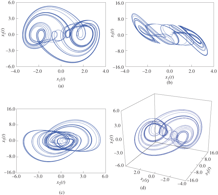
Figure 2.8 Chaotic behaviors of fractional-order Arneodo system (2.49): (a)  –
– plane; (b)
  –
– plane; (c)
  –
– plane; (d)
  –
– –
– space.
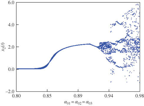
Figure 2.9 Bifurcation diagram of fractional-order Arneodo system (2.49) for  .
.
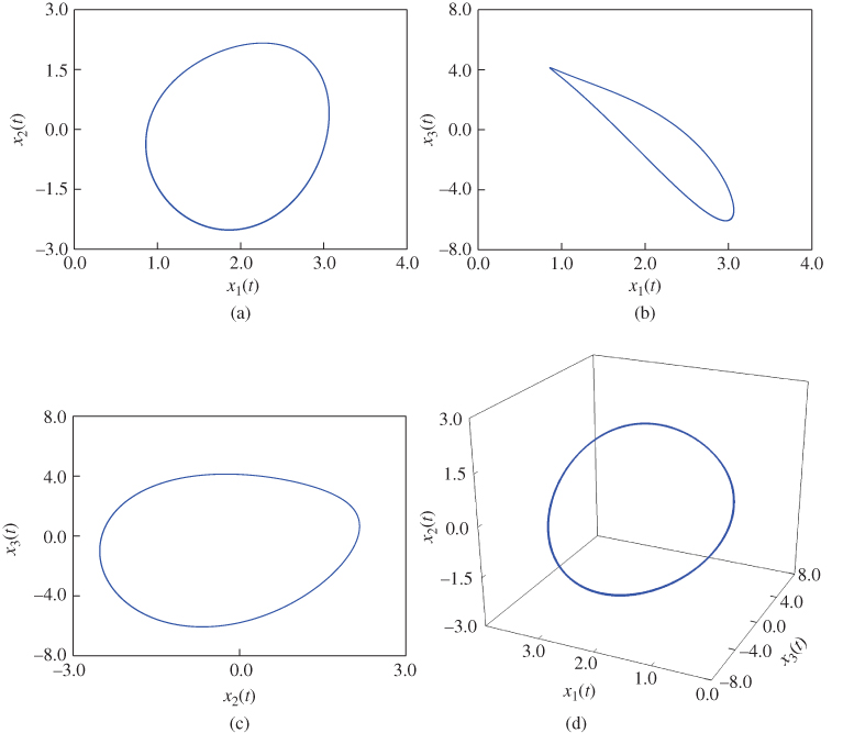
Figure 2.10 Dynamic characteristic of one cycle for fractional-order Arneodo system (2.49): (a)  –
– plane; (b)
  –
– plane; (c)
  –
– plane; (d)
  –
– –
– space.
2.2.5 Fractional-Order Lotka–Volterra System
A two-predator and one-prey generalization of the Lotka–Volterra system was proposed by Samardzija and Greller [182]. Its fractional-order model is given as follows [164]:

where ![]() ,
, ![]() , and
, and ![]() are fractional orders,
are fractional orders, ![]() ,
, ![]() , and
, and ![]() are system state variables, and
are system state variables, and ![]() ,
, ![]() , and
, and ![]() are system parameters. For fractional orders chosen as
are system parameters. For fractional orders chosen as ![]() , system parameters given by
, system parameters given by ![]() ,
, ![]() , and
, and ![]() and initial conditions chosen as
and initial conditions chosen as ![]() ,
, ![]() , and
, and ![]() , the simulation results of the fractional-order Lotka–Volterra system are presented in Figure 2.11. Furthermore, the bifurcation diagram for
, the simulation results of the fractional-order Lotka–Volterra system are presented in Figure 2.11. Furthermore, the bifurcation diagram for ![]() is presented in Figure 2.12. Following the bifurcation diagram (Figure 2.12), the chaotic dynamic characteristic for
is presented in Figure 2.12. Following the bifurcation diagram (Figure 2.12), the chaotic dynamic characteristic for ![]() is shown in Figure 2.13.
is shown in Figure 2.13.

Figure 2.11 Chaotic behaviors of fractional-order Lotka–Volterra system (2.50): (a)  –
– plane; (b)
  –
– plane; (c)
  –
– plane; (d)
  –
– –
– space.

Figure 2.12 Bifurcation diagram of fractional-order Lotka–Volterra system (2.50) for  .
.

Figure 2.13 Dynamic behaviors of fractional-order Lotka–Volterra system (2.50): (a)  –
– plane; (b)
  –
– plane; (c)
  –
– plane; (d)
  –
– –
– space.
2.2.6 Fractional-Order Financial System
Ma and Chen [183] gave a simplified finance model. According to the integer-order finance model, the fractional-order financial system is described as follows [8]:

where ![]() ,
, ![]() , and
, and ![]() are fractional orders,
are fractional orders, ![]() ,
, ![]() , and
, and ![]() are system state variables, and
are system state variables, and ![]() ,
, ![]() , and
, and ![]() are system parameters. For fractional orders chosen as
are system parameters. For fractional orders chosen as ![]() , system parameters given by
, system parameters given by ![]() and
and ![]() , and initial conditions chosen as
, and initial conditions chosen as ![]() ,
, ![]() , and
, and ![]() , the simulation results of the fractional-order financial system are given in Figure 2.14. Furthermore, the bifurcation diagram for
, the simulation results of the fractional-order financial system are given in Figure 2.14. Furthermore, the bifurcation diagram for ![]() is presented in Figure 2.15. Following the bifurcation diagram (Figure 2.15), the dynamic characteristic of one cycle for
is presented in Figure 2.15. Following the bifurcation diagram (Figure 2.15), the dynamic characteristic of one cycle for ![]() is shown in Figure 2.16.
is shown in Figure 2.16.

Figure 2.14 Chaotic behaviors of fractional-order financial system (2.51): (a)  –
– plane; (b)
  –
– plane; (c)
  –
– plane; (d)
  –
– –
– space.

Figure 2.15 Bifurcation diagram of fractional-order financial system (2.51) for  .
.

Figure 2.16 Dynamic characteristic of one cycle for fractional-order financial system (2.51): (a)  –
– plane; (b)
  –
– plane; (c)
  –
– plane; (d)
  –
– –
– space.
2.2.7 Fractional-Order Newton–Leipnik System
The Newton–Leipnik system is described by a nonlinear differential equation in [164]. By considering the fractional calculus, the fractional-order Newton-Leipnik system is given by Sheu et al. [184] as follows:

where ![]() ,
, ![]() , and
, and ![]() are fractional orders,
are fractional orders, ![]() ,
, ![]() , and
, and ![]() are system state variables, and
are system state variables, and ![]() and
and ![]() are system parameters. For fractional orders chosen as
are system parameters. For fractional orders chosen as ![]() , system parameters given by
, system parameters given by ![]() and
and ![]() , and initial conditions chosen as
, and initial conditions chosen as ![]() ,
, ![]() , and
, and ![]() , the simulation results of the fractional-order Newton–Leipnik system are shown in Figure 2.17. Furthermore, the bifurcation diagram for
, the simulation results of the fractional-order Newton–Leipnik system are shown in Figure 2.17. Furthermore, the bifurcation diagram for ![]() is presented in Figure 2.18. Following the bifurcation diagram (Figure 2.18), the chaotic dynamic characteristic for
is presented in Figure 2.18. Following the bifurcation diagram (Figure 2.18), the chaotic dynamic characteristic for ![]() is shown in Figure 2.19.
is shown in Figure 2.19.

Figure 2.17 Chaotic behaviors of fractional-order Newton–Leipnik system (2.52): (a)  –
– plane; (b)
  –
– plane; (c)
  –
– plane; (d)
  –
– –
– space.

Figure 2.18 Bifurcation diagram of fractional-order Newton–Leipnik system (2.52) for  .
.

Figure 2.19 Dynamic behaviors of fractional-order Newton–Leipnik system (2.52): (a)  –
– plane; (b)
  –
– plane; (c)
  –
– plane; (d)
  –
– –
– space.
2.2.8 Fractional-Order Duffing System
The fractional-order Duffing system is written as follows [164]:

where ![]() and
and ![]() are fractional orders,
are fractional orders, ![]() and
and ![]() are system state variables, and
are system state variables, and ![]() ,
, ![]() , and
, and ![]() are system parameters. For fractional orders chosen as
are system parameters. For fractional orders chosen as ![]() and
and ![]() , system parameters given by
, system parameters given by ![]() ,
, ![]() , and
, and ![]() , and initial conditions chosen as
, and initial conditions chosen as ![]() and
and ![]() , the simulation results of the fractional-order Duffing system are given in Figure 2.20. Furthermore, the bifurcation diagram for
, the simulation results of the fractional-order Duffing system are given in Figure 2.20. Furthermore, the bifurcation diagram for ![]() is presented in Figure 2.21. Following the bifurcation diagram (Figure 2.21), the dynamic characteristic of one cycle for
is presented in Figure 2.21. Following the bifurcation diagram (Figure 2.21), the dynamic characteristic of one cycle for ![]() is shown in Figure 2.22.
is shown in Figure 2.22.

Figure 2.20 Simulation result of fractional-order Duffing system (2.53).

Figure 2.21 Bifurcation diagram of fractional-order Duffing system (2.53) for  .
.

Figure 2.22 Dynamic characteristic of one cycle for fractional-order Duffing system (2.53).
2.2.9 Fractional-Order Lü System
The Lü system [185] is known as a bridge between the Lorenz system [178] and the Chen system [186]. Its fractional-order differential equation is described as follows [187]:

where ![]() ,
, ![]() , and
, and ![]() are fractional orders,
are fractional orders, ![]() ,
, ![]() , and
, and ![]() are system state variables, and
are system state variables, and ![]() ,
, ![]() , and
, and ![]() are system parameters. For fractional orders chosen as
are system parameters. For fractional orders chosen as ![]() , system parameters given by
, system parameters given by ![]() ,
, ![]() , and
, and ![]() , and initial conditions chosen as
, and initial conditions chosen as ![]() ,
, ![]() , and
, and ![]() , the simulation results of the fractional-order Lü system are presented in Figure 2.23. Furthermore, the bifurcation diagram for
, the simulation results of the fractional-order Lü system are presented in Figure 2.23. Furthermore, the bifurcation diagram for ![]() is presented in Figure 2.24. Following the bifurcation diagram (Figure 2.24), the dynamic characteristic of one cycle for
is presented in Figure 2.24. Following the bifurcation diagram (Figure 2.24), the dynamic characteristic of one cycle for ![]() is shown in Figure 2.25.
is shown in Figure 2.25.

Figure 2.23 Chaotic behaviors of fractional-order Lü system (2.54): (a)  –
– plane; (b)
  –
– plane; (c)
  –
– plane; (d)
  –
– –
– space.

Figure 2.24 Bifurcation diagram of fractional-order Lü system (2.54) for  .
.

Figure 2.25 Dynamic characteristic of one cycle for fractional-order Lü system (2.54): (a)  –
– plane; (b)
  –
– plane; (c)
  –
– plane; (d)
  –
– –
– space.
2.2.10 Fractional-Order Three-Dimensional System
On the basis of the fractional-order Lorenz system [179], a three-dimensional fractional-order system is written as follows [188]:

where ![]() ,
, ![]() , and
, and ![]() are fractional orders,
are fractional orders, ![]() ,
, ![]() , and
, and ![]() are system state variables, and
are system state variables, and ![]() ,
, ![]() , and
, and ![]() are system parameters. For fractional orders chosen as
are system parameters. For fractional orders chosen as ![]() ,
, ![]() , and
, and ![]() , system parameters given by
, system parameters given by ![]() ,
, ![]() , and
, and ![]() , and initial conditions chosen as
, and initial conditions chosen as ![]() ,
, ![]() , and
, and ![]() , the simulation results of the fractional-order three-dimensional system are shown in Figure 2.26. Furthermore, the bifurcation diagram for
, the simulation results of the fractional-order three-dimensional system are shown in Figure 2.26. Furthermore, the bifurcation diagram for ![]() is presented in Figure 2.27. Following the bifurcation diagram (Figure 2.27), the dynamic characteristic of one cycle for
is presented in Figure 2.27. Following the bifurcation diagram (Figure 2.27), the dynamic characteristic of one cycle for ![]() is shown in Figure 2.28.
is shown in Figure 2.28.
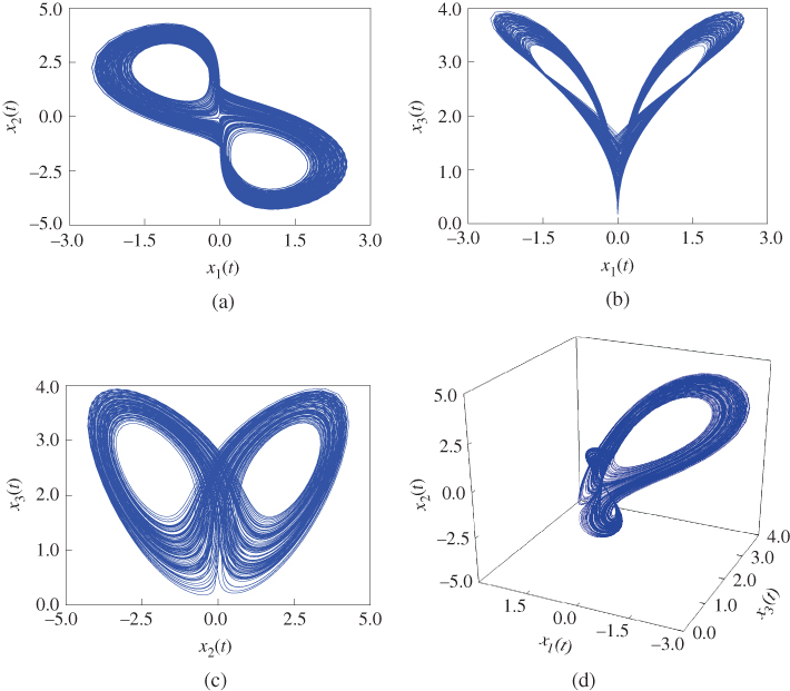
Figure 2.26 Chaotic behaviors of fractional-order three-dimensional system (2.55): (a)  –
– plane; (b)
  –
– plane; (c)
  –
– plane; (d)
  –
– –
– space.

Figure 2.27 Bifurcation diagram of fractional-order three-dimensional system (2.55) for  .
.

Figure 2.28 Dynamic characteristic of one cycle for fractional-order three-dimensional system (2.55): (a)  –
– plane; (b)
  –
– plane; (c)
  –
– plane; (d)
  –
– –
– space.
2.2.11 Fractional-Order Hyperchaotic Oscillator
The fractional-order hyperchaotic oscillator is described by the following form [189]:

where ![]() ,
, ![]() ,
, ![]() ,
, ![]() , and
, and ![]() are fractional orders,
are fractional orders, ![]() ,
, ![]() ,
, ![]() , and
, and ![]() are system state variables, and
are system state variables, and ![]() ,
, ![]() ,
, ![]() ,
, ![]() ,
, ![]() , and
, and ![]() are system parameters. For fractional orders chosen as
are system parameters. For fractional orders chosen as ![]() , system parameters given by
, system parameters given by ![]() ,
, ![]() ,
, ![]() ,
, ![]() ,
, ![]() , and
, and ![]() , and initial conditions chosen as
, and initial conditions chosen as ![]() ,
, ![]() ,
, ![]() , and
, and ![]() , the simulation results of the fractional-order hyperchaotic oscillator are given in Figure 2.29. Furthermore, the bifurcation diagram for
, the simulation results of the fractional-order hyperchaotic oscillator are given in Figure 2.29. Furthermore, the bifurcation diagram for ![]() is presented in Figure 2.30. According to the bifurcation diagram (Figure 2.30), the dynamic characteristic of one cycle for
is presented in Figure 2.30. According to the bifurcation diagram (Figure 2.30), the dynamic characteristic of one cycle for ![]() is shown in Figure 2.31.
is shown in Figure 2.31.

Figure 2.29 Chaotic behaviors of fractional-order hyperchaotic oscillator (2.56): (a)  –
– plane; (b)
  –
– plane; (c)
  –
– plane; (d)
  –
– –
– space.
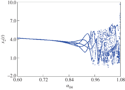
Figure 2.30 Bifurcation diagram of fractional-order hyperchaotic oscillator (2.56) for  .
.

Figure 2.31 Dynamic characteristic of one cycle for fractional-order hyperchaotic oscillator (2.56): (a)  –
– plane; (b)
  –
– plane; (c)
  –
– plane; (d)
  –
– –
– space.
2.2.12 Fractional-Order Four-Dimensional Hyperchaotic System
The fractional version of the four-dimensional hyperchaotic system is given by the following [190]:

where ![]() ,
, ![]() ,
, ![]() , and
, and ![]() are fractional orders,
are fractional orders, ![]() ,
, ![]() ,
, ![]() , and
, and ![]() are system state variables, and
are system state variables, and ![]() ,
, ![]() ,
, ![]() ,
, ![]() , and
, and ![]() are system parameters. For fractional orders chosen as
are system parameters. For fractional orders chosen as ![]() , system parameters given by
, system parameters given by ![]() ,
, ![]() ,
, ![]() ,
, ![]() , and
, and ![]() , and initial conditions chosen as
, and initial conditions chosen as ![]() ,
, ![]() ,
, ![]() , and
, and ![]() , the simulation results of the fractional-order four-dimensional hyperchaotic system are presented in Figure 2.32. Furthermore, the bifurcation diagram for
, the simulation results of the fractional-order four-dimensional hyperchaotic system are presented in Figure 2.32. Furthermore, the bifurcation diagram for ![]() is presented in Figure 2.33. Following the bifurcation diagram (Figure 2.33), the dynamic characteristic of one cycle for
is presented in Figure 2.33. Following the bifurcation diagram (Figure 2.33), the dynamic characteristic of one cycle for ![]() is shown in Figure 2.34.
is shown in Figure 2.34.

Figure 2.32 Chaotic behaviors of fractional-order four-dimensional hyperchaotic system (2.57): (a)  –
– plane; (b)
  –
– plane; (c)
  –
– plane; (d)
  –
– –
– space.

Figure 2.33 Bifurcation diagram of fractional-order four-dimensional hyperchaotic system (2.57) for 
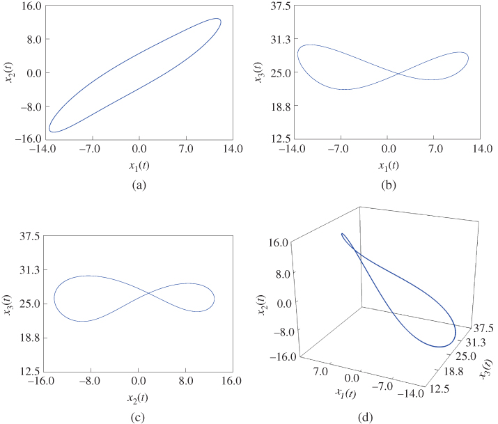
Figure 2.34 Dynamic characteristic of one cycle for fractional-order four-dimensional hyperchaotic system (2.57): (a)  –
– plane; (b)
  –
– plane; (c)
  –
– plane; (d)
  –
– –
– space.
2.2.13 Fractional-Order Hyperchaotic Cellular Neural Network
The model of a fractional-order hyperchaotic cellular neural network can be written as follows [191]:

where ![]()
![]() ,
, ![]() ,
, ![]() , and
, and ![]() are fractional orders,
are fractional orders, ![]() ,
, ![]() ,
, ![]() , and
, and ![]() are system state variables, and
are system state variables, and ![]() ,
, ![]() , and
, and ![]() are system parameters. For fractional orders chosen as
are system parameters. For fractional orders chosen as ![]() , system parameters given by
, system parameters given by ![]() ,
, ![]() , and
, and ![]() , and initial conditions chosen as
, and initial conditions chosen as ![]() ,
, ![]() ,
, ![]() , and
, and ![]() , the simulation results of a fractional-order hyperchaotic cellular neural network are shown in Figure 2.35. Furthermore, the bifurcation diagram for
, the simulation results of a fractional-order hyperchaotic cellular neural network are shown in Figure 2.35. Furthermore, the bifurcation diagram for ![]() is presented in Figure 2.36. Following the bifurcation diagram (Figure 2.36), the chaotic dynamic characteristic for
is presented in Figure 2.36. Following the bifurcation diagram (Figure 2.36), the chaotic dynamic characteristic for ![]() is shown in Figure 2.37.
is shown in Figure 2.37.

Figure 2.35 Chaotic behaviors of fractional-order hyperchaotic cellular neural network (2.58): (a)  –
– plane; (b)
  –
– plane; (c)
  –
– plane; (d)
  –
– –
– space.

Figure 2.36 Bifurcation diagram of fractional-order hyperchaotic cellular neural network (2.58) for  .
.

Figure 2.37 Dynamic behaviors of fractional-order hyperchaotic cellular neural network (2.58): (a)  –
– plane; (b)
  –
– plane; (c)
  –
– plane; (d)
  –
– –
– space.
2.3 Conclusion
In this chapter, principle definitions of the fractional integral and fractional derivatives have been given. Furthermore, some lemmas have been introduced, along with results on the stability of fractional-order systems. Finally, some fractional-order systems have been listed: fractional-order Lorenz system, fractional-order van der Pol oscillator, fractional-order Genesio–Tesi system, fractional-order Arneodo system, fractional-order Lotka–Volterra system, fractional-order financial system, fractional-order Newton–Leipnik system, fractional-order Duffing system, fractional-order Lü system, fractional-order three-dimensional system, fractional-order hyperchaotic oscillator, fractional-order four-dimensional hyperchaotic system, and fractional-order hyperchaotic cellular neural network.