
Chapter 4
Design of Fractional-Order Controllers for Nonlinear Chaotic Systems and Some Applications
4.1 Fractional-Order Control for a Novel Chaotic System Without Equilibrium
4.1.1 Problem Statement
In this section, a novel chaotic system will be proposed by only considering the straight-line position ![]() and the pitch angle
and the pitch angle ![]() of the two-wheeled self-balancing robot of Googol Technology. A mathematical model related to the two-wheeled self-balancing robot of Googol Technology was established by Son and Anh [208]. The linear mathematical model for
of the two-wheeled self-balancing robot of Googol Technology. A mathematical model related to the two-wheeled self-balancing robot of Googol Technology was established by Son and Anh [208]. The linear mathematical model for ![]() and
and ![]() of the two-wheeled self-balancing robot of Googol Technology is described in the form of
of the two-wheeled self-balancing robot of Googol Technology is described in the form of

where ![]() denotes the pitch torque.
denotes the pitch torque.
To transform the linear mathematical model into a chaotic system, we consider ![]() as a nonlinear term
as a nonlinear term ![]() , which will be given in next section.
, which will be given in next section.
Considering the nonlinear function ![]() and the control input
and the control input ![]() , Equation (4.1) can be described as
, Equation (4.1) can be described as

where the control input ![]() .
.
In this chapter, we aim to construct a novel chaotic system without equilibrium and to develop a fractional-order control scheme, so that the stabilization of the whole closed-loop system, including the novel chaotic system and the control input, is realized based on the designed control strategy. Under the designed fractional-order controller, the state variables of the closed-loop system are asymptotically stable.
In Chapter 2, three types of fractional calculus definitions were introduced. According to the different types of fractional calculus, some important control schemes have been proposed. ML stability theorems have been proposed [209–211] for fractional-order systems. The stability theorem was developed for fractional differential system with the RL derivative [212–214]. In this chapter, a control scheme based on the fractional-order controller will be designed using the Caputo definition (2.17), with the lower limit of the integral as ![]() and fractional order
and fractional order ![]() .
.
4.1.2 Design of Chaotic System and Circuit Implementation
In this chapter, a novel chaotic system without equilibrium has been constructed based on the linear mathematical model (4.1) of the two-wheeled self-balancing robot. For this case, the proposed novel chaotic system can be regarded as an open-loop system of the system (4.2). Furthermore, the chaotic circuit is designed to address the physical realizability of the proposed chaotic system.
4.1.2.1 A Novel Chaotic System
From Equation (4.2), the novel chaotic system can be described as follows:

where ![]() is the state vector of the nonlinear system with
is the state vector of the nonlinear system with ![]() ,
, ![]() ,
, ![]() and
and ![]() . The nonlinear function
. The nonlinear function ![]() is given by
is given by
where ![]() and
and ![]() are constants. When
are constants. When ![]() and
and ![]() , we obtain the Lyapunov exponents
, we obtain the Lyapunov exponents ![]() ,
, ![]() ,
, ![]() , and
, and ![]() by calculating for the initial conditions
by calculating for the initial conditions ![]() . Obviously, the system (4.3) is a chaotic system under such case because
. Obviously, the system (4.3) is a chaotic system under such case because ![]() ,
, ![]() ,
, ![]() , and
, and ![]() . On the basis of the system (4.3) and the mentioned parameter values, the simulation results are further presented as shown in Figure 4.1. In addition, to further reflect the properties of chaos, the Poincaré map is shown in Figure 4.2.
. On the basis of the system (4.3) and the mentioned parameter values, the simulation results are further presented as shown in Figure 4.1. In addition, to further reflect the properties of chaos, the Poincaré map is shown in Figure 4.2.

Figure 4.1 Chaotic behaviors of the novel chaotic system: (a)  –
– plane; (b)
  –
– plane; (c)
  –
– plane; (d)
  –
– –
– space.

Figure 4.2 Poincaré map in the  –
– plane.
To solve the equilibrium of system (4.3), we let ![]() ,
, ![]() ,
, ![]() , and
, and ![]() ; this gives
; this gives

According to system (4.5), we obtain that there is no equilibrium in system (4.3). Furthermore, we ensure that the system (4.3) is dissipative with the following exponential contraction rate of the exponential function ![]() :
:
with

4.1.2.2 Circuit Implementation
To further illustrate the physical realizability of the proposed novel chaotic system (4.3), the system circuit is designed. By using resistors, capacitors, and operational amplifiers (TL082), the designed circuit of the chaotic system is shown in Figure 4.3. According to Figure 4.3, the circuit equation of the chaotic system is described as follows:

By comparing system (4.3) with system (4.8), it can be deduced that all resistance values ![]() ,
, ![]() ,
, ![]() ,
, ![]() ,
, ![]() ,
, ![]() ,
, ![]() ,
, ![]() ,
, ![]() ,
, ![]() ,
, ![]() , and
, and ![]() are 10 k
are 10 k![]() ,
, ![]() and
and ![]() are 1 M
are 1 M![]() ,
, ![]() ,
, ![]() , and
, and ![]() are 21.7514 k
are 21.7514 k![]() ,
, ![]() ,
, ![]() , and
, and ![]() are 5.251715 k
are 5.251715 k![]() ,
, ![]() is 42.2474 k
is 42.2474 k![]() ,
, ![]() is 8.031303 k
is 8.031303 k![]() ,
, ![]() is 435.02849 k
is 435.02849 k![]() , and
, and ![]() is 105.0343 k
is 105.0343 k![]() . The voltage values are
. The voltage values are ![]() V and
V and ![]() V. To speed up the circuit response time, we make a time-scale transformation by multiplying by a factor of 100 on the right-hand-side of system (4.3); the capacitance values
V. To speed up the circuit response time, we make a time-scale transformation by multiplying by a factor of 100 on the right-hand-side of system (4.3); the capacitance values ![]() ,
, ![]() ,
, ![]() , and
, and ![]() are then 10 nF. In Figure 4.3,
are then 10 nF. In Figure 4.3, ![]() are operational amplifiers, where
are operational amplifiers, where ![]() is a unity-gain multiplier.
is a unity-gain multiplier.
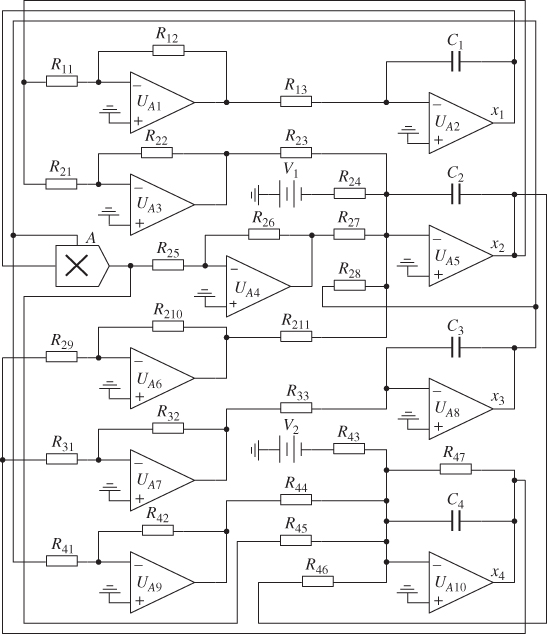
Figure 4.3 Circuit of the novel chaotic system (4.3).
From the designed circuit of the chaotic system (4.3), experimental circuit phase portraits are presented in Figure 4.4. Comparing Figure 4.1 and Figure 4.4, we observe that there is consistency between numerical simulations and circuit experimental simulations; the circuit simulation results prove the physical realizability of the proposed novel chaotic system (4.3).
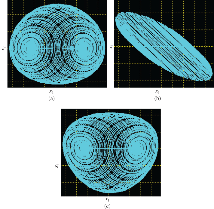
Figure 4.4 Chaotic behaviors of the chaotic circuit: (a)  –
– plane; (b)
  –
– plane; (c)
  –
– plane.
4.1.3 Design of Fractional-Order Controller and Stability Analysis
In this section, the control scheme will be proposed for the whole closed-loop system including the constructed chaotic system (4.3) and a fractional-order controller. The goal is to guarantee the stabilization of the closed-loop system under the proposed fractional-order controller.
From Equations (4.3) and (4.4), the chaotic system can be rewritten as
where

with ![]() the state vector, and
the state vector, and

According to the chaotic system (4.9) and considering the control input ![]() , the corresponding system can be written in the following form:
, the corresponding system can be written in the following form:
where ![]() is the designed fractional-order control input.
is the designed fractional-order control input.
Based on the state-feedback control method, the controller ![]() is defined as
is defined as
where ![]() is a design control gain matrix and the fractional order satisfies
is a design control gain matrix and the fractional order satisfies ![]() .
.
According to Equations (4.10) and (4.11), one has
To render the stabilization of the closed-loop system (4.12) under the proposed controller (4.11), the following assumption is required.
The fractional-order controller based control scheme for the system (4.10) can be summarized in the following theorem.
4.1.4 Numerical Simulation
In this section, to illustrate and verify the effectiveness of the proposed control scheme, the closed-loop system (4.12) is analyzed. Furthermore, we use the proposed control scheme to stabilize chaotic systems with equilibrium, such as the Chen system [216], Genesio's system [217] and the hyperchaotic Lorenz system [218].
4.1.4.1 Novel Chaotic System
Combining the novel chaotic system (4.3) with the designed controller (4.11), we have the following:

The equilibrium of system (4.23) is obtained by solving ![]() ,
, ![]() ,
, ![]() , and
, and ![]() , which gives the following:
, which gives the following:

According to system (4.24), we obtain that ![]() is the equilibrium of the system (4.23). Furthermore, when the design parameters
is the equilibrium of the system (4.23). Furthermore, when the design parameters ![]() ,
, ![]() ,
, ![]() , and
, and ![]() satisfy
satisfy ![]() ,
, ![]() ,
, ![]() , and
, and ![]() , we can guarantee that the equilibrium
, we can guarantee that the equilibrium ![]() is a stable equilibrium based on the stability analysis method of the equilibrium [164]. From Equation (4.23), we have
is a stable equilibrium based on the stability analysis method of the equilibrium [164]. From Equation (4.23), we have

which implies that ![]() satisfies Assumption 4.1. On the basis of Theorem 4.1 and the pole placement technique, the feedback control gain matrix
satisfies Assumption 4.1. On the basis of Theorem 4.1 and the pole placement technique, the feedback control gain matrix ![]() and the order
and the order ![]() are chosen as
are chosen as
From this discussion, we have ![]() ,
, ![]() , and
, and ![]() ; the conditions of Theorem 4.1 are satisfied. The simulation results are shown in Figure 4.5 and Figure 4.6. According to the numerical simulation results, the closed-loop system (4.23) is asymptotically stable, which implies that the proposed control scheme works effectively.
; the conditions of Theorem 4.1 are satisfied. The simulation results are shown in Figure 4.5 and Figure 4.6. According to the numerical simulation results, the closed-loop system (4.23) is asymptotically stable, which implies that the proposed control scheme works effectively.

Figure 4.5 Numerical simulation results of the system (4.23).

Figure 4.6 Control inputs of the system (4.23).
4.1.4.2 Chaotic Systems with Equilibrium
To further illustrate the effectiveness of the developed control scheme in this chapter, we use the proposed control scheme (4.11) to control the Chen system [216], Genesio's system [217], and the hyperchaotic Lorenz system [218]. We first analyze the following dynamic model of the Chen system [216]:

From Equation (4.11), the control input ![]() is designed for the Chen system as follows:
is designed for the Chen system as follows:

Invoking system (4.27), we have

where ![]() . According to Equation (4.29), the nonlinear function in (4.27) can satisfy Assumption 4.1. Therefore, the Chen system (4.27) can be stabilized to zero by choosing appropriate parameters
. According to Equation (4.29), the nonlinear function in (4.27) can satisfy Assumption 4.1. Therefore, the Chen system (4.27) can be stabilized to zero by choosing appropriate parameters ![]() ,
, ![]() , and
, and ![]() .
.
Genesio's system is written as follows:

To control Genesio's system (4.30), the control input ![]() can be designed based on Equation (4.11), as follows:
can be designed based on Equation (4.11), as follows:

From system (4.30), we obtain

where ![]() .
.
The nonlinear function in system (4.30) can satisfy Assumption 4.1 based on Equation (4.32). Thus, Genesio's system (4.30) can be stabilized to zero under the appropriate parameters ![]() ,
, ![]() , and
, and ![]() .
.
The hyperchaotic Lorenz system is given as follows:

Combining the hyperchaotic Lorenz system (4.33) and the control law (4.11), the control input ![]() is written as follows:
is written as follows:

According to system (4.33), we have

where ![]() .
.
On the basis of Equation (4.35), Assumption 4.1 is satisfied for the nonlinear function in system (4.33). By choosing appropriate parameters ![]() ,
, ![]() ,
, ![]() , and
, and ![]() , the stabilization of the hyperchaotic Lorenz system (4.33) can be realized.
, the stabilization of the hyperchaotic Lorenz system (4.33) can be realized.
According to the this discussion and analysis, we obtain that the Chen system (4.27), Genesio's system (4.30), and the hyperchaotic Lorenz system (4.33) are controlled using the control scheme described in this chapter. For the numerical simulation of the Chen system (4.27), we choose the control parameters ![]() ,
, ![]() , and
, and ![]() , the initial conditions
, the initial conditions ![]() , and the fractional order
, and the fractional order ![]() . For the numerical simulation of Genesio's system (4.30), we set the control parameters
. For the numerical simulation of Genesio's system (4.30), we set the control parameters ![]() ,
, ![]() , and
, and ![]() , the initial conditions
, the initial conditions ![]() , and the fractional order
, and the fractional order ![]() . In the numerical simulation of the hyperchaotic Lorenz system (4.33), the control parameters are designed as
. In the numerical simulation of the hyperchaotic Lorenz system (4.33), the control parameters are designed as ![]() ,
, ![]() ,
, ![]() , and
, and ![]() , the initial conditions are assumed as
, the initial conditions are assumed as ![]() , and the fractional order is chosen as
, and the fractional order is chosen as ![]() .
.
On the basis of the given simulation conditions, the numerical results are presented in Figure 4.7, Figure 4.8, Figure 4.9, Figure 4.10, Figure 4.11, and Figure 4.12 for the Chen system (4.27), Genesio's system (4.30), and the hyperchaotic Lorenz system (4.33), respectively. The control results of the Chen system (4.27) are shown in Figure 4.7. It is shown that good control performance is obtained under the designed controller (4.28). Figure 4.8 presents the control inputs (4.28). The numerical simulation results of Genesio's system (4.30) are given in Figure 4.9 and Figure 4.10. Figure 4.9 and Figure 4.10 show that the controller (4.31) can stabilize Genesio's system (4.30) well. Finally, Figure 4.11 and Figure 4.12 show that the fractional-order controller (4.34) can control all state variables of the hyperchaotic Lorenz system (4.33) to the origin. Therefore, all the simulation results show that the fractional-order controller can also control the chaotic and hyperchaotic systems with equilibrium.

Figure 4.7 Stabilization of Chen system (4.27).

Figure 4.8 Control inputs of Chen system (4.27).

Figure 4.9 Stabilization of Genesio's system (4.30).

Figure 4.10 Control inputs for Genesio's system (4.30).

Figure 4.11 Stabilization of hyperchaotic Lorenz system (4.33).
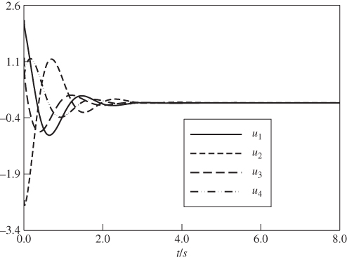
Figure 4.12 Control inputs for hyperchaotic Lorenz system (4.33).
4.2 Application of Chaotic System without Equilibrium in Image Encryption
On the basis of the proposed chaotic system without equilibrium (4.3), the image encryption scheme is developed in this section. Generally, the security will be better if the encrypted image is very fuzzy. The analysis of the effect of encryption for the image encryption scheme [219] will be given by the following four aspects:
- 1. Histogram analysis. The histogram of the image is an important statistical characteristic of the image, and is the approximation of the density function of the gray image.
- 2. Correlation of two adjacent pixels. Each pixel of any image has a high correlation with its adjacent pixels, either horizontally, vertically, or diagonally. The correlation of two adjacent pixels can be presented in a diagram. Furthermore, the correlation coefficient of each pair of pixels can also be calculated via the following formulas [219]:
4.36
 4.37
4.37 4.38
4.38 4.39
4.39
- where
 and
and  are the gray values of two adjacent pixels in the image,
  denotes the expectation,
  denotes the variance,
  denotes the covariance,
  denotes the total number of adjacent pairs of pixels, and
  denotes the correlation coefficient of two adjacent pixels.
 - 3. Anti-attack ability of image encryption scheme. The anti-attack ability is analyzed by the recovery level of the broken image.
- 4. Sensitivity of keys. A good encryption algorithm should be sensitive to a secret key. Small changes in the decryption key will lead to failed decrypted images.
4.2.1 Image Encryption Scheme
According to the chaotic sequences of the chaotic system without equilibrium (4.3), pixel substitution, and pixel value scrambling methods, the image encryption scheme is given for an image (the size is ![]() , where
, where ![]() and
and ![]() represent the rows and columns of the image). The steps for the encryption algorithm are as follows:
represent the rows and columns of the image). The steps for the encryption algorithm are as follows:
- 1. Assume a random value
 as the initial condition of the chaotic system without equilibrium (4.3). Then four groups of chaotic time sequences with good stochastic properties are obtained.
 - 2. Select a group of chaotic time sequences from the given four groups of chaotic time sequences. Then a subsequence is designed, based on the selected chaotic time sequence, where the size of the subsequence is
 . Moreover, a new sequence of integers is given according to the subsequence, where the sequence of integers is set as
  .
. - 3. The pixel values of the origin image are loaded. Then the time sequence of pixel values (
 ) is then translated into the binary serialization.
 - 4. The elements in
 and
and  are handled by the xor method for each of
  and
and  . Then a new time sequence
  is obtained and the binary serialization is translated into decimal format.
 - 5. Select another group of chaotic time sequence from the given four groups of chaotic time sequences. Then a subsequence
 is designed based on the selected chaotic time sequence, where the size of the subsequence is
  . Furthermore, the subsequence
  is further tackled by
  .
. - 6. A group of new natural sequences
 is added. Then the elements in
  are initialized, that is,
  . The following processing procedure for the element
  is given as: (1) select the element
  in
in  . Then the
  th element in
  is exchanged by the
  th element; (2) the exchanged element is moved back
  positions.
 - 7. A new time sequence
 is obtained based on the given time sequences
  and
and  . Then the new time sequence
  is translated into a replacement matrix
  .
. - 8. Setting the replacement matrix
 as the mapping address table, and the address of elements for the matrix
  are rearranged. Then a new pixel matrix
  is obtained. Therefore, the image encryption scheme is realized.
4.2.2 Histogram Analysis
We assume that the size of the original image is ![]() and the range of gray levels for each pixel is 0–255. The original image is presented in Figure 4.13a. The initial condition of the chaotic system without equilibrium (4.3) is chosen as
and the range of gray levels for each pixel is 0–255. The original image is presented in Figure 4.13a. The initial condition of the chaotic system without equilibrium (4.3) is chosen as ![]() . Then four groups of chaotic time sequences are obtained by numerical simulation. The chaotic time sequence
. Then four groups of chaotic time sequences are obtained by numerical simulation. The chaotic time sequence ![]() –
–![]() is selected as the subsequence
is selected as the subsequence ![]() and the original image is encrypted using the pixel substitution method. Furthermore, we select the chaotic time sequence
and the original image is encrypted using the pixel substitution method. Furthermore, we select the chaotic time sequence ![]() –
–![]() as the replacement matrix
as the replacement matrix ![]() . Finally, the fully encrypted image is shown in Figure 4.14a.
. Finally, the fully encrypted image is shown in Figure 4.14a.

Figure 4.13 (a) Original image; (b) corresponding gray distribution histogram.

Figure 4.14 (a) Encrypted image; (b) corresponding gray distribution histogram.
Figure 4.13b and Figure 4.14b show the corresponding gray distributions of the original image and the image encrypted using the designed algorithm, respectively. The results from Figure 4.13 and Figure 4.14 indicate that the image encryption scheme is valid, that is: (i) the encrypted image in Figure 4.14a is totally different from the original image (Figure 4.13a); (ii) the statistical characteristics of the encrypted image in Figure 4.14b are also different from those of the original image (Figure 4.13b).
4.2.3 Correlation of Two Adjacent Pixels
Figure 4.15a and Figure 4.15b show the correlations of two horizontal adjacent pixels for the original and encrypted images, respectively. Also, Table 4.1 presents the correlation coefficient of the encrypted image and the original image. It is obvious that the correlation coefficient of the encrypted image in any direction is approximately equal to zero. As a result, the correlated relationship is very low.
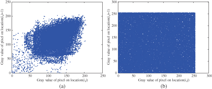
Figure 4.15 Correlations of two horizontal adjacent pixels: (a) in original image; (b) in encrypted image.
Table 4.1 Correlation coefficients in original and encrypted images
| Original image | Encrypted image | |
| Horizontal | 0.7467 | |
| Vertical | 0.8319 | |
| Diagonal | 0.3468 |
4.2.4 Anti-Attack Ability of Image Encryption Scheme
Take the cropping attack as the analysis object. We assume that the intermediate region is attacked (the size is ![]() ) or that the boundary area is attacked (the size is
) or that the boundary area is attacked (the size is ![]() ), as shown in Figure 4.16. Then the decrypted image, as shown in Figure 4.17, can also present the shape of the original image. Furthermore, Figure 4.17 is further handled by a median filter algorithm. The restored image is shown in Figure 4.18, which shows that a better restored effect is presented. It is obvious from Figure 4.16, Figure 4.17, and Figure 4.18 that the attacked image can also be restored using the designed image encryption scheme.
), as shown in Figure 4.16. Then the decrypted image, as shown in Figure 4.17, can also present the shape of the original image. Furthermore, Figure 4.17 is further handled by a median filter algorithm. The restored image is shown in Figure 4.18, which shows that a better restored effect is presented. It is obvious from Figure 4.16, Figure 4.17, and Figure 4.18 that the attacked image can also be restored using the designed image encryption scheme.

Figure 4.16 Attacked images.

Figure 4.17 Decrypted images.

Figure 4.18 Restored images.
4.2.5 Sensitivity Analysis of Key
Key sensitivity is an essential property for any good cryptosystem, and ensures the security of the cryptosystem against brute-force attacks. The encrypted image produced by the cryptosystem should be sensitive to the secret key. That is to say, if the attacker uses two slightly different keys to decrypt the same plain image, the two encrypted images should be completely independent of each other [220]. The encrypted image of Figure 4.14a is decrypted using the secret keys ![]() and the decrypted image is shown in Figure 4.19a. Now, we attempt to decrypt the encrypted image using other keys (the key is assumed as
and the decrypted image is shown in Figure 4.19a. Now, we attempt to decrypt the encrypted image using other keys (the key is assumed as ![]() ). The decrypted image is shown in Figure 4.19b. Obviously, the decrypted image is different from the original image (Figure 4.19a). We can conclude that the decrypted image cannot be restored via incorrect keys.
). The decrypted image is shown in Figure 4.19b. Obviously, the decrypted image is different from the original image (Figure 4.19a). We can conclude that the decrypted image cannot be restored via incorrect keys.

Figure 4.19 Decryption attempt results using: (a) correct key; (b) incorrect key.
4.3 Synchronization Control for Fractional-Order Nonlinear Chaotic Systems
4.3.1 Problem Description
According to the Caputo fractional derivative (2.17), the fractional-order system can be written as [221]
where ![]() is the state vector,
is the state vector, ![]() is a constant matrix, and the fractional order is
is a constant matrix, and the fractional order is ![]() . If
. If ![]() denotes another state vector, the nonlinear functions
denotes another state vector, the nonlinear functions ![]() and
and ![]() satisfy the following condition:
satisfy the following condition:
where ![]() and
and ![]() denote the linear and nonlinear parts, respectively.
denote the linear and nonlinear parts, respectively.
This section aims to develop a synchronization control scheme based on the fractional-order controller. On the basis of the designed controller, the response system can synchronize the drive system well under the proper conditions.
4.3.2 Design of Synchronization Controller
Since synchronization can be applied to secure communications and signal processing, synchronization control is an important problem for investigations of fractional-order chaotic systems. Synchronization of fractional-order chaotic systems is realized by designing an appropriate fractional-order controller.
The fractional-order chaotic system (4.40) is taken as the master system, and the slave system is defined as
where ![]() denotes the control input vector.
denotes the control input vector.
Define the synchronization error as
where ![]() .
.
According to Equations (4.40) (4.42), and (4.43), the synchronization error system can be described as
Furthermore, the control input is designed by
where ![]() denotes the design matrix,
denotes the design matrix, ![]() is an invertible matrix,
is an invertible matrix, ![]() denotes a diagonal matrix, and
denotes a diagonal matrix, and ![]() denotes an identity matrix.
denotes an identity matrix.
This synchronization control scheme for fractional-order nonlinear chaotic systems can be summarized in the following theorem.
4.3.3 Simulation Examples
To illustrate the effectiveness of the designed synchronization controller, the fractional-order Chen system [223] and the fractional-order Lorenz system [179] are investigated.
4.3.3.1 Fractional-Order Chen System
The fractional-order Chen system is given as follows [223]:

where ![]() is the fractional order,
is the fractional order, ![]() ,
, ![]() , and
, and ![]() are system parameters, and
are system parameters, and ![]() ,
, ![]() , and
, and ![]() are system state variables. The parameters are chosen as
are system state variables. The parameters are chosen as ![]() ,
, ![]() and
and ![]() , the fractional order is given by
, the fractional order is given by ![]() , and the initial conditions are chosen as
, and the initial conditions are chosen as ![]() . Then the chaotic behaviors of the fractional-order Chen system (4.55) are shown in Figure 4.20.
. Then the chaotic behaviors of the fractional-order Chen system (4.55) are shown in Figure 4.20.

Figure 4.20 Chaotic behaviors of fractional-order Chen system: (a)  –
– plane; (b)
  –
– plane; (c)
  –
– plane; (d)
  –
– –
– space.
Furthermore, the fractional-order Chen system (4.55) can be written as

The fractional-order Chen system (4.55) is taken as the master system, and the slave system is described by

where ![]() ,
, ![]() , and
, and ![]() are system state variables and
are system state variables and ![]() ,
, ![]() , and
, and ![]() are control inputs.
are control inputs.
According to Equations (4.56) and (4.57), we obtain

On the basis of Equation (4.58), we have

From Equation (4.59), we obtain

Referring to the designed controller of Equations (4.45) (4.56) (4.57), and (4.59), on the basis of Equation (4.58), we have

where ![]() is a design control matrix. If the conditions in Theorem 4.2 are satisfied, the error system (4.61) will tend to zero. Then synchronization is realized between the master system (4.56) and the slave system (4.57).
is a design control matrix. If the conditions in Theorem 4.2 are satisfied, the error system (4.61) will tend to zero. Then synchronization is realized between the master system (4.56) and the slave system (4.57).
For the numerical simulation, we choose the design parameters as ![]() ,
, ![]() , and
, and ![]() and the initial conditions as
and the initial conditions as ![]() and
and ![]() . Then we have
. Then we have

According to Equation (4.57), we obtain that ![]() and
and ![]() , thus the conditions in Theorem 4.2 are satisfied. The numerical results are shown in Figure 4.21 and Figure 4.22 under the proposed synchronization control scheme. The state synchronization results of the master system (4.56) and the slave system (4.57) are given in Figure 4.21a–c. It is shown that the good synchronization performance is achieved. Figure 4.22 shows that the synchronization errors
, thus the conditions in Theorem 4.2 are satisfied. The numerical results are shown in Figure 4.21 and Figure 4.22 under the proposed synchronization control scheme. The state synchronization results of the master system (4.56) and the slave system (4.57) are given in Figure 4.21a–c. It is shown that the good synchronization performance is achieved. Figure 4.22 shows that the synchronization errors ![]() ,
, ![]() , and
, and ![]() are convergent. According to the simulation results, the master system (4.56) and the slave system (4.57) are synchronous under the designed fractional-order controller (4.45). Therefore, the proposed synchronization control scheme is valid for fractional-order chaotic systems.
are convergent. According to the simulation results, the master system (4.56) and the slave system (4.57) are synchronous under the designed fractional-order controller (4.45). Therefore, the proposed synchronization control scheme is valid for fractional-order chaotic systems.

Figure 4.21 Synchronization results of state variables of two fractional-order Chen systems: (a)  and
and  ; (b)
; (b)  and
and  ; (c)
; (c)  and
and  .
.

Figure 4.22 Synchronization errors  ,
,  , and
, and  of two fractional-order Chen systems.
4.3.3.2 Fractional-Order Lorenz System
According to Equation (2.46), the fractional-order Lorenz system can be written as follows:

where ![]() is the fractional order,
is the fractional order, ![]() ,
, ![]() , and
, and ![]() are system state variables, and
are system state variables, and ![]() ,
, ![]() , and
, and ![]() are system parameters. For the fractional order given by
are system parameters. For the fractional order given by ![]() , system parameters chosen as
, system parameters chosen as ![]() ,
, ![]() , and
, and ![]() , and initial conditions chosen as
, and initial conditions chosen as ![]() , the simulation results of the fractional-order Lorenz system are shown in Figure 2.1.
, the simulation results of the fractional-order Lorenz system are shown in Figure 2.1.
From Equation (4.63), we have

The fractional-order Lorenz system (4.64) is taken as the master system, and the slave system is given as

where ![]() ,
, ![]() , and
, and ![]() are system state variables and
are system state variables and ![]() ,
, ![]() , and
, and ![]() are control inputs.
are control inputs.
From Equations (4.64) and (4.65), we obtain

According to Equation (4.66), we have

On the basis of Equation (4.67), we obtain

Invoking Equations (4.45) (4.64)–(4.66), and (4.67), we have

where ![]() is a design matrix. The error system (4.69) will tend to zero when the conditions in Theorem 4.2 are satisfied. Then synchronization is realized between the master system (4.64) and the slave system (4.65).
is a design matrix. The error system (4.69) will tend to zero when the conditions in Theorem 4.2 are satisfied. Then synchronization is realized between the master system (4.64) and the slave system (4.65).
For the numerical simulation, the design parameters are designed as ![]() ,
, ![]() , and
, and ![]() , the initial conditions are chosen as
, the initial conditions are chosen as ![]() and
and ![]() . Then we have
. Then we have

According to Equation (4.70), we obtain that ![]() and
and ![]() , thus the conditions in Theorem 4.2 are satisfied. According to the proposed synchronization control scheme, the numerical results are given in Figure 4.23 and Figure 4.24. The state synchronization results are presented in Figure 4.23a–c. From Figure 4.23, the synchronization performance is good. Figure 4.24 shows that the synchronization errors
, thus the conditions in Theorem 4.2 are satisfied. According to the proposed synchronization control scheme, the numerical results are given in Figure 4.23 and Figure 4.24. The state synchronization results are presented in Figure 4.23a–c. From Figure 4.23, the synchronization performance is good. Figure 4.24 shows that the synchronization errors ![]() ,
, ![]() , and
, and ![]() are convergent. On the basis of the simulation results, the master system (4.64) and the slave system (4.65) are synchronous, based on the designed fractional-order controller (4.45). Therefore, the proposed synchronization control scheme is effective for fractional-order chaotic systems.
are convergent. On the basis of the simulation results, the master system (4.64) and the slave system (4.65) are synchronous, based on the designed fractional-order controller (4.45). Therefore, the proposed synchronization control scheme is effective for fractional-order chaotic systems.

Figure 4.23 Synchronization results of state variables of two fractional-order Lorenz systems: (a)  and
and  ; (b)
; (b)  and
and  ; (c)
; (c)  and
and  .
.

Figure 4.24 Synchronization errors  ,
,  , and
, and  of two fractional-order Lorenz systems.
4.3.4 Application of Synchronization Control Scheme in Secure Communication
In this section, the synchronization control scheme is applied in secure communication through the chaotic masking technology. The information signal can be concealed and recovered.
To illustrate the effectiveness of the synchronization control scheme in secure communication, synchronization of the fractional-order Chen system is applied in secure communication based on the chaotic masking technology [224] illustrated in Figure 4.25. For secure communication, we assume that the master system (4.55) is regarded as the transmitter of the secure communication system and the slave system (4.57) is regarded as the acceptor of the secure communication system. Then we use the chaotic synchronization signals ![]() and
and ![]() to realize encryption transmission of the information signal
to realize encryption transmission of the information signal ![]() . If synchronization is achieved for the chaotic signals
. If synchronization is achieved for the chaotic signals ![]() and
and ![]() , the synchronization error
, the synchronization error ![]() will tend to zero and the recovered signal
will tend to zero and the recovered signal ![]() can be described as
can be described as

Figure 4.25 Chaotic masking technology.
According to Equation (4.71), we can obtain that the encrypted signal can be recovered by the acceptor of the secure communication system when synchronization is realized. For the numerical simulation, we assume that the information signal ![]() . The mixture signal of
. The mixture signal of ![]() and
and ![]() can be written as
can be written as ![]() . Then the secure communication system is realized based on synchronization of the fractional-order Chen system. The simulation results are presented in Figure 4.26. From Figure 4.26, we can see that the information signal
. Then the secure communication system is realized based on synchronization of the fractional-order Chen system. The simulation results are presented in Figure 4.26. From Figure 4.26, we can see that the information signal ![]() can be masked by the chaotic signal
can be masked by the chaotic signal ![]() . Furthermore, the acceptor can recover the encrypted signal well. Thus, the effectiveness of the synchronization control scheme is illustrated in secure communication.
. Furthermore, the acceptor can recover the encrypted signal well. Thus, the effectiveness of the synchronization control scheme is illustrated in secure communication.

Figure 4.26 Simulation results: (a) information signal  ; (b) mixture signal
  ; (c) recovered signal
  ; (d) error signal
  .
.
4.4 Conclusion
In this chapter, a novel chaotic system without equilibrium has been proposed. The Lyapunov exponents and the Poincaré map of the proposed chaotic system have been given. Meanwhile, the dissipativeness of the new chaotic system has been illustrated. The chaotic circuit has been designed to demonstrate the physical realizability of the novel chaotic system. In addition, on the basis of the Gronwall inequality, the Laplace transform, the ML function, and the state-feedback method, a stability theorem for the chaotic system without equilibrium has been given. The designed controller has been developed to realize the stabilization of the closed-loop systems. The proposed control scheme has been developed to control the chaotic and hyperchaotic systems with equilibrium, i.e. the Chen system, Genesio's system, and the hyperchaotic Lorenz system. An image encryption scheme has been developed by using the proposed chaotic system without equilibrium. Furthermore, on the basis of the Gronwall inequality, the Laplace transform, the ML function, and the state-feedback method, a synchronization control scheme has been given for a class of fractional-order nonlinear systems. The synchronization control scheme has been used to realize the synchronization of two fractional-order Chen systems and two fractional-order Lorenz systems, respectively. Numerical simulation results further illustrate the effectiveness of the developed synchronization control scheme. Finally, the proposed synchronization control scheme has been applied in secure communication through chaotic masking technology and the effectiveness of synchronization control scheme in secure communication is illustrated.