Chapter 8
The Transform and Data Menus
In This Chapter
![]() Sorting your cases in different ways
Sorting your cases in different ways
![]() Using some data (and not other data) with Select and Split
Using some data (and not other data) with Select and Split
![]() Combining counting and case identifying
Combining counting and case identifying
![]() Recoding variable content to new values
Recoding variable content to new values
![]() Grouping data in bins
Grouping data in bins
After you get your raw data into SPSS, you may find that it contains errors or that it isn’t organized the way you’d like. A way to alleviate these problems is by making modifications to your data, configuring the values into a form that’s easier to work with and read. This chapter contains some methods you can use to modify your data without losing any information.
A related problem is that you may want to analyze only some of your data, or you may want to perform the analysis more than once. For example, you may want to do a separate analysis for new customers and established customers. You may even want to select the good complete data and avoid the incomplete messy data. It’s all about massaging the data after it’s in SPSS and making it ready to work for you.
Sorting Cases
You can change the order of your cases (rows) so they appear in just about any order you want. You sort them by comparing the values you entered for your variables. The following example uses the Cars.sav dataset. We sort with two variables, or sort keys. The initial sort of the data will simply be by Car ID.
 You don’t need to limit your sorting to one or two sort keys. You can have a third and fourth key, or more, if necessary, but these keys come into effect only when the keys sorted before them hold identical values. In most cases, two sort keys are plenty to get what you want.
You can sort based on variables of any type simply by selecting the variables as keys. For example:
-
Choose File ⇒ Open ⇒ Data and open the Cars.sav file.
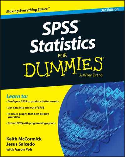
The result is the presentation of a collection of apparently unsorted cases shown in Figure 8-1.
-
Choose Data ⇒ Sort Cases.
The dialog box is shown in Figure 8-2.
-
Choose the variables Country of Origin and Horsepower, in that order.
The result is shown in Figure 8-3.
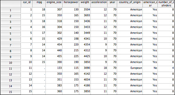
Figure 8-1: The data unsorted, as it’s loaded directly from the data file.
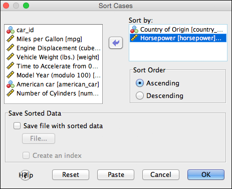
Figure 8-2: The data sorted by horsepower.
Figure 8-3: The data sorted alphabetically by Country of Origin and then by Horsepower.
 Sorting data is strictly for the way you want it to appear in the table. The order in which the data is displayed never affects the analysis. You can get a quick sense of what’s going on by sorting your data, but in the end, it isn’t a substitute for a proper analysis in the output window.
The order of the sort keys is important. In the preceding example, if Horsepower had been chosen as the first key and Country of Origin as the second, we would’ve gotten different results.
 If you need to sort using only one variable, you can just right-click the column name.
Selecting the Data You Want to Look At
A very powerful way of manipulating your data is to turn some data “off,” while leaving other data “on.” In this example, we analyze just European cars, without having to delete anything. SPSS even makes it easy to keep track of what’s being counted, averaged, analyzed, and so on, and what’s turned “off.”
-
Choose File ⇒ Open ⇒ Data and open the Cars.sav file.
If Cars.sav is already open, that’s fine, but we’ll be starting with the data sorted on Car ID.
- Choose Data ⇒ Sort Cases.
-
Choose the variable Car ID.
Now that the data has been sort on Car ID, we can select the European cars so we can do our analyses just on them.
-
Choose Data ⇒ Select Cases.
The dialog box is shown in Figure 8-4.
-
Select the If Condition Is Satisfied radio button and then click the If button (refer to Figure 8-4).
You’re taken to the dialog box in Figure 8-5.
Now we can specify the selection criteria.
- Type country_of_origin = 2, in the expression box and then click OK.
We have just told SPSS that we want to only select those cases that have a value of 2 on the variable country of origin. It’s important that you type the number 2, and not “European” because the actual stored value is 2 and the labeled data is “European.”
Figure 8-6 shows the final result. Note the slashes over some of the Row IDs. This shows that the American cars are being ignored (for the time being) and that only the European cars are being analyzed.
From this point forward, every piece of output that you generate will use only the European cars until you turn the Select off. There is a button to return to All Cases in the original menu (refer to Figure 8-4.)
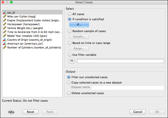
Figure 8-4: The Select Cases dialog box.
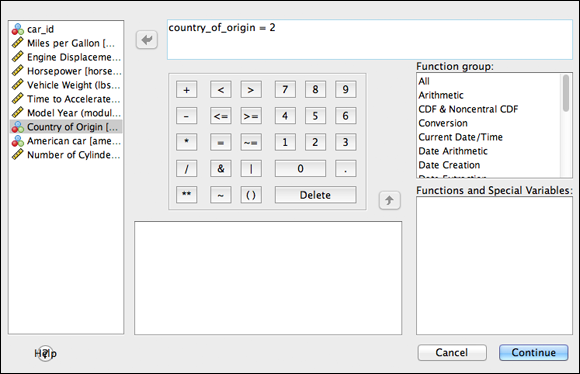
Figure 8-5: The If dialog box.
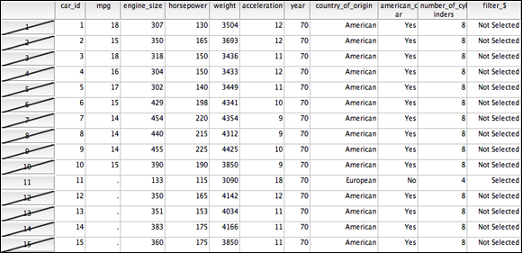
Figure 8-6: The data sorted, indicating selected and unselected cases.
You should always use values and labels for your category values, as is done with the Country of Origin variable in this dataset. This is the way SPSS likes it, and you don’t want to make SPSS grumpy, do you? Try typing in just strings, and you’re likely to get some errors and random happenings. SPSS’s bad mood could soon become your own. Use values and labels to keep everyone happy.
If you wanted to select complete data on a variable (horsepower, for example) you can use the following phrase in the IF formula area: not(missing(horsepower)).
Sometimes the values like 1, 2, and 3 are showing in the data window, and sometimes the labels like American, European, and Japanese are showing. There is an easy way to switch back and forth. The button shown in Figure 8-7 appears in the toolbar in the data window. It toggles back and forth between values and labels.

Figure 8-7: The dataset toolbar button for toggling between values and labels.
Splitting Your Data for Easier Analysis
Under some conditions, you can use an even more powerful version of what we’ve just illustrated with SELECT. For instance, sometimes you might want to run a series of analyses on one group of cases, and then you can select another group of cases and rerun the same analyses on them. The Split file procedure allows you to select each group in turn, one at a time, and run all your analyses on each separate group.
-
Choose File ⇒ Open ⇒ Data and open the Cars.sav file.
If Cars.sav is already open, that’s fine, but we’ll be starting with the data sorted on Car ID. Make sure that the SELECT in the last example has been turned off by returning your SELECT status to All Cases.
-
Choose Data ⇒ Split File.
The dialog box is shown in Figure 8-8.
-
Choose Country_of_Origin as the Compare Groups variable and click OK.
Your data window won’t have slashes as in the case of SELECT. Until we run some output, it won’t be clear that anything has changed.
- Choose Analyze ⇒ Descriptive Statistics ⇒ Frequencies.
-
Choose Number of Cylinders and click OK.
The resulting output, shown in Figure 8-9, is broken down by Country of Origin. We can stay in this mode as long as we like. Spending hours with a SPLIT on is not unheard of when producing tables, charts, and statistics for each of your groups.
It’s important when you’re done with your SPLIT (or a SELECT) that you turn them off. The option to turn off your SPLIT is the Analyze All Cases, Do Not Produce Groups radio button in the original menu shown in Figure 8-8.
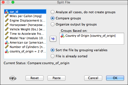
Figure 8-8: Completed Split File dialog box.
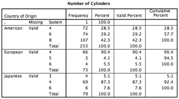
Figure 8-9: The results of the FREQUENCY while in SPLIT mode.
In the far bottom right of the data window there is an indicator that tells you whether you currently have a SPLIT or SELECT operation turned on.
Counting Case Occurrences
If your data is being used to keep track of multiple similar occurrences — such as people who subscribe to any combination of three different magazines, or eggs produced with something other than a single yolk — you can automatically generate a count of the occurrences for each case. SPSS automates the process of creating a new variable and counting the values for you. You specify what value(s) cause a variable to qualify, and SPSS counts the number of qualifying variables from among those you choose. You must have a number of variables that all normally take the same range of values. For example, if you have a number of expenses for each case, you could have SPSS count the number of expenses that exceed a certain threshold.
In the following example, people are listed as subscribers or nonsubscribers to three magazines, which are named simply mag1, mag2, and mag3. The following steps generate a total of the number of subscriptions for each person:
-
Choose Open ⇒ File ⇒ Data and open the magazines.sav file.
This file can be downloaded from the book’s companion website at
www.dummies.com/go/spss. The screen shown in Figure 8-10 appears. - Choose Transform ⇒ Count Values Within Cases.
The screen shown in Figure 8-11 appears.
-
Select the name of every variable you want to use in the count, and then click the arrow to move them from the panel on the left to the panel on the right labeled Variables. Give your new variable a name.
This operation works only with numerics because it must perform numeric matches on the values. If you want, you can come up with both a name and a label to be assigned to the variable that this process creates. In this example, the name is count and the label is Count of subscriptions, as shown in Figure 8-12.
-
Click the Define Values button.
The window shown in Figure 8-13 appears. In this window, we’ve decided to count, from among the selected variables, those with the numeric value of 1 — which in our example is the value that signifies a subscription.
As you can see in the figure, the total can also be based on missing values and ranges of values. In the ranges, you can specify both the high and low values, or you can specify one end of the range and have the other end be either the largest or the smallest value in the set. In fact, you can select a number of criteria, and SPSS will check each variable against all of them.
-
Select a criterion value you want to use, and then click the Add button to move it to the panel on the right labeled Values to Count. Repeat as needed to define all your criteria.
The new variable will contain a count of the variables that you named that have a value that matches at least one of the criteria you specified. Each case is counted separately.
-
Click Continue.
You return to the Count Occurrences of Values within Cases screen (refer to Figure 8-11).
-
Click If.
The window shown in Figure 8-14 appears.
-
Define your expression.
By default, all cases are included, but you can specify criteria here to exclude some cases. To do so, select the Include If Case Satisfies Condition option and, in the text box below, define an expression that specifies the values you want to accept. Then only the values for which the expression is true are considered as candidates for a count greater than 0. You can use any of the variables in the expression. And by using the number pad, the operator buttons, and the function selection, you can construct any expression you want.
- Click the Continue button to have SPSS accept your definition. Otherwise (as we did for this simple example), click Cancel and all cases are considered.
-
Click the OK button and the new field, along with its counts, is generated.
The result is the new variable named count, as shown in Figure 8-15.
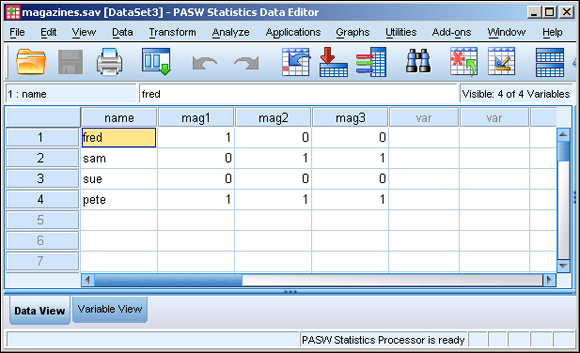
Figure 8-10: Each magazine has the value 1 for a subscriber and 0 for a nonsubscriber.
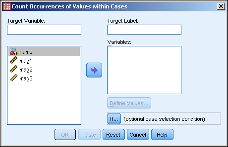
Figure 8-11: The initial value-counting window.
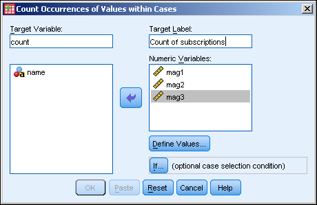
Figure 8-12: The chosen variables to be counted, and the name of the new variable.
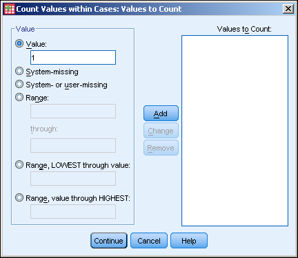
Figure 8-13: Define the criteria that determine which values are included in the count.
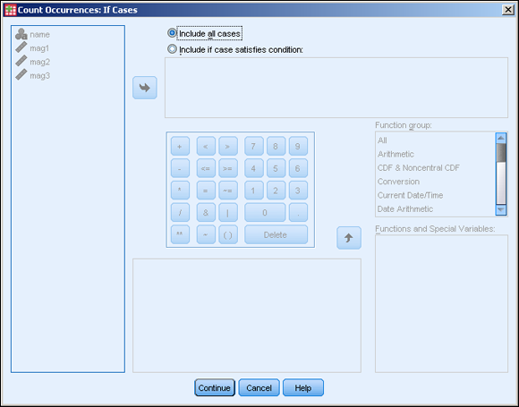
Figure 8-14: Define arithmetic expressions that determine which values are included in the count.
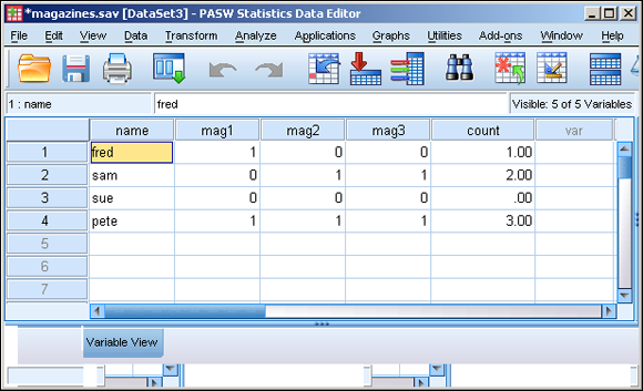
Figure 8-15: A new variable containing the total number of subscriptions per case.
Recoding Variables
You can have SPSS change specific values to other specific values according to rules you give it. You can change almost any value to anything else. For example, if you have Yes and No represented by 5 and 6, you could recode the values into 1 and 2. You can recode the values in place without creating a new variable, or you can create a new variable and recode values into it. You may want to do this to correct errors or to make the data easier to use.
 When you’re recoding values without creating a new variable to receive the new numbers, be sure you store a safety copy of your data before you start. Changes to your data can’t be automatically reversed; you could destroy information. For this reason, avoid Recode into Same Variables unless you’re sure that you want to use it. The main reason to consider it is if you want to change a bunch of variables all at once. Better to stick with Recode into Different Variables.
Recoding into different variables
Maybe you don’t want to overwrite the existing values, but you’d like to have the recoded data available. This is always a safe way to recode. You can always delete the original later if you don’t need it. The following steps create the recoded values and are stored in a new variable:
- Load the rsvp.sav dataset, as shown in Figure 8-16, and choose Transform ⇒ Recode into Different Variables.
- In the left panel, select the Response variable holding the values you want to change. Using the arrow in the center, move the variable name to the panel in the center.
-
On the right, in the Output Variable area, enter a name (attending) and label (Attending or not) for a new variable.
For the output variable, you can choose a new variable name (so a new variable is created) or choose an existing variable name and have its values overwritten.
- Click the Change button and the output variable is defined, as shown in Figure 8-17.
- Click the Old and New Values button.
-
Define the recoding.
Enter an existing value into the Old Value text box and the value you want it to become in the New Value text box. Then click the Add button to add them to the Old-->New list (as shown in Figure 8-18). Be sure to map all values — even the ones that don’t change — because you’re creating a new variable and it has no preset values.
- Click Continue.
-
Click OK.
The results appear, as shown in Figure 8-19. Notice that the numbers all have two digits to the right of the decimal point. This may or may not be what you want, but the new variable was created automatically, and that’s part of the default.
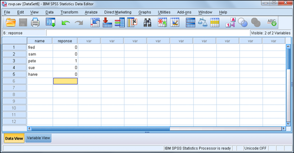
Figure 8-16: The rsvp.sav data file.
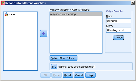
Figure 8-17: Name the variable to receive the recoded values.
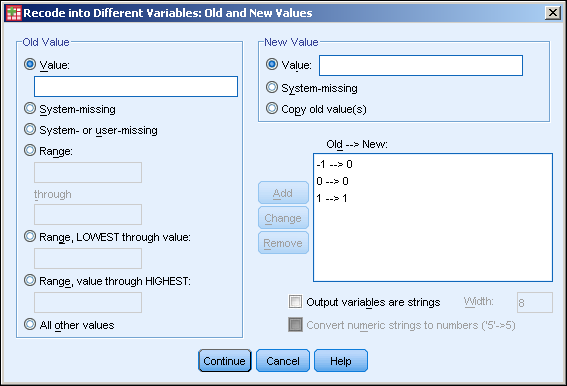
Figure 8-18: All possible values recoded for a new variable.
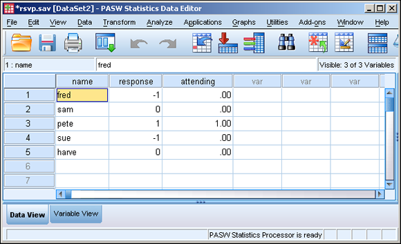
Figure 8-19: Values recoded into a new variable.
Automatic recoding
Automatic recoding converts values into something you can use in computations. For example, if you have a list of automobile names, automatic recoding converts those names into numbers so you can perform an analysis on the pattern of numbers. Automatic recoding gives you a numeric handle on data that could otherwise elude analysis.
To perform automatic recoding, you select options and set the names in a single dialog box. To see an example of automatic recoding in action, follow these steps:
- Load rsvp.sav (refer to Figure 8-16).
-
Choose Transform ⇒ Automatic Recode.
The Automatic Recode dialog box appears.
- In the panel on the left, select the name of the variable you want to recode. Then click the arrow in the middle to move the variable to the panel on the right.
- In the New Name text box, enter the name of the variable to receive the recoded values.
-
Click the Add New Name button.
The name you entered appears in the panel above the new name, as shown in Figure 8-20.
-
Click OK.
Recoding takes place. The result is similar to that shown in Figure 8-21, where the new variable is named index.
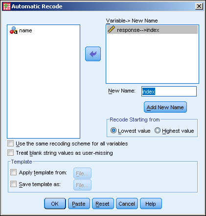
Figure 8-20: The dialog box for automatic recoding.
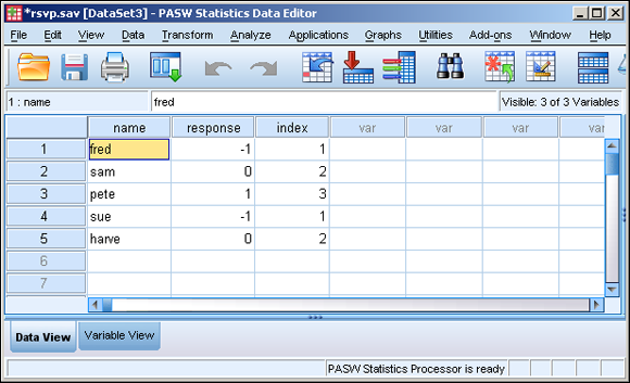
Figure 8-21: The result of automatically recoding name into index.
The values in the new variable, index, come about from sorting the values of the original variable and then assigning numbers to them in that order. If the input values are a string of characters instead of the digits of numbers, the strings are sorted alphabetically (well, almost: uppercase letters come before lowercase).
In the Automatic Recode window (refer to Figure 8-20), you can see the choice for recoding the values with new numbers that start with either the lowest value or the highest value. The new numeric values will be the same either way; they’re just assigned in the opposite order.
At the bottom of the Automatic Recode window are two choices for the creation of a template file. This is so you can save a file — called a template file — that holds a record of the recoding patterns. That way, if you need to recode more data with the same variable names, the new input values will be compared against the previous encoding and be given appropriate values so that the two data files can be merged and the data will all fit. For example, if you have brand names or part numbers in your data, the recoding will be consistent with the original values because it will be assigned the same pattern of recoded values.
Binning
If you’re using a scale variable that contains a range of values, you can create groups of those values and organize them into bins. For example, you could use the ages of a number of people and put each one in its own bin — one bin for ages 0 to 20, another bin for ages 21 to 40, and so on. You can specify the size and content of bins in several ways. The actual binning process is automatic.
The following steps take you through an example of the binning process by dividing salaries into bins:
Choose File ⇒ Open ⇒ Data and load the salaries.sav file.
This file is available for download as described in the introduction. This file contains a list of ID numbers with a salary for each one, as shown in Figure 8-22.
-
Choose Transform ⇒ Visual Binning.
The dialog box shown in Figure 8-23 appears.
-
Select Current Salary in the panel on the left; then click the arrow in the center of the window to move the name of the variable to the panel on the right.
Click Continue.
A bar graph displaying the range of values of the salaries appears in the center, as shown in Figure 8-24.
- Click the Make Cutpoints button. A dialog box appears; here you can specify the size of each bin and the number of bins.
-
Select the points at which you want to have the data cut into parts to create the bins.
In this example, we divided the data into even percentiles of numbers of cases — that is, each bin will contain the same number of cases, as shown in Figure 8-25. Notice that four cutpoints divide the data into five bins, each holding 20% of the cases. We could’ve chosen to divide the data into equal-width intervals — that is, each bin would contain a range of the same magnitude, which would put different numbers of cases in each bin. Also, the cutpoints could have been based on standard deviations, which would create two cutpoints, dividing the data into the three bins — one each of low, medium, and high capacity.
- Click the Apply button, and the cutpoints appear as vertical lines on the bar graph, as shown in Figure8-26 You may click the Make Cutpoints button repeatedly and cut the data different ways until you get the cutpoints the way you like. Any new cutpoints you define replace any previous ones.
-
Enter a name for a new variable to contain the binning information.
You enter the name in the Binned Variable text box. The default label for the new variable appears in the text box to the right of the name. You can change this if you want. The bins are created and numbered from 1 to 5, but if you select the Reverse Scale option (in the lower-right corner), the numbering will be from 5 to 1.
-
Click OK.
The new variable is created and filled with the bin values, as shown in Figure 8-27.
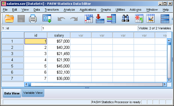
Figure 8-22: A list of employee ID numbers and the salaries corresponding to them.
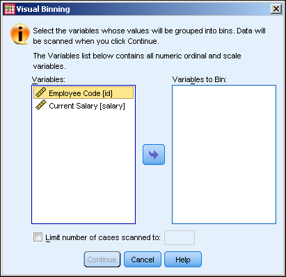
Figure 8-23: Select the name of the variable to be binned.
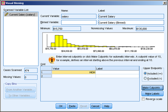
Figure 8-24: How the binning will be done.
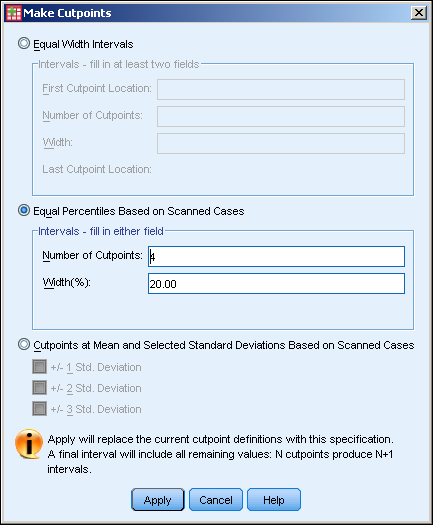
Figure 8-25: Specify how you want the data divided into bins.
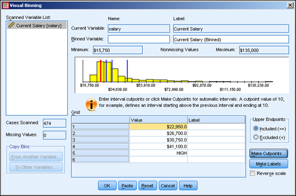
Figure 8-26: A bar graph of the data with cutpoints for binning.
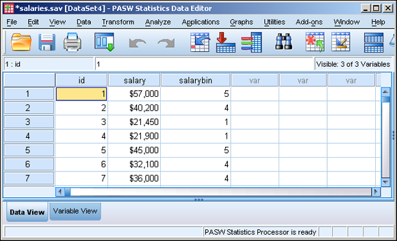
Figure 8-27: The new variable containing the bin numbers.
The binning is now complete and you can use the new data for further analysis. One thing you can do quickly and easily is display a summary of the contents of your bins. Simply follow these steps:
- With the window in Figure 8-27 still on the screen, choose Transform ⇒ Optimal Binning.
-
Select variable names on the left and click the arrow buttons to move the variables. Move Current Salary to Variables to Bin and move Current Salary (binned) to Optimize Bins with Respect To, as shown in Figure 8-28.
The variable in the Optimize Bins with Respect To text box doesn’t have to be a variable from a previous binning operation. It can be any variable that contains a collection of values sufficient for being separated into bins.
-
Click OK.
The output is generated, as shown in Figure 8-29.
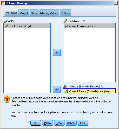
Figure 8-28: Select the bin variable and the optimizing variable.
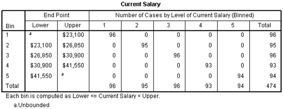
Figure 8-29: The output from optimal binning.
Any variable with properly distributed values can be used as the basis of optimal binning. In Figure 8-29, the numbers 1 through 5 across the top are the values of the new binning variable created and stored as part of the data. The numbers 1 through 5 down the left of the graph are the result of the new binning action. The chart lets you see clearly the range of values that make up each bin.