17.3. Common performance problems

The rapid advance of technology together with falling component prices has meant a lot of database design and administration problems can be buried beneath a pile of memory and fast multicore CPUs. In some cases, this may be a valid option; however, throwing hardware at a problem is usually the least effective means of improving performance, with the greatest performance gains usually coming from good design and maintenance strategies.

In this section, we'll address a number of common performance problems and the wait types and performance counters applicable to each. We'll start with procedure cache bloating before moving on to CPU pressure, index-related memory pressure, disk bottlenecks, and blocking.

17.3.1. Procedure cache bloating

In chapter 7 we covered the various SQL Server components that utilize system memory, with the two largest components being the data cache and the procedure cache. The data cache is used for storing data read from disk, and the procedure cache is used for query compilation and execution plans.

Each time a query is submitted for processing, SQL Server assesses the contents of the procedure cache for an existing plan that can be reused. If none is found, SQL Server generates a new plan, storing it in the procedure cache for (possible) later reuse.

Reusing existing plans is a key performance-tuning goal for two reasons: first, we reduce the CPU overhead in compiling new plans, and second, the size of the procedure cache is kept as small as possible. A smaller procedure cache enables a larger data cache, effectively boosting RAM and reducing disk I/O.

The most effective way of controlling the growth of the procedure cache is reducing the incidence of unparameterized ad hoc queries.

Ad hoc queries

A common attribute among poorly performing SQL Server systems with a large procedure cache is the volume of ad hoc SQL that's submitted for execution. For example, consider the following queries:^[]

^[] In the following examples, we'll run DBCC FREEPROCCACHE before each set of queries to clear the contents of the procedure cache, enabling the cache usage to be easily understood.

DBCC FREEPROCCACHE
    GO
    SELECT * FROM Production.Product WHERE ProductNumber = 'FW-5160'
    GO
    SELECT * FROM Production.Product WHERE ProductNumber = 'HN-1220'
    GO
    SELECT * FROM Production.Product WHERE ProductNumber = 'BE-2908'
    GO

All three of these queries are exactly the same with the exception of the ProductNumber parameter. Using the sys.dm_exec_cached_plans and sys.dm_exec_sql_text views and functions, let's inspect the procedure cache to see how SQL Server has cached these queries. Figure 17.7 displays the results.

Figure 17.7. Unparameterized SQL results in multiple ad hoc compiled plans.
 

As per figure 17.7, SQL Server has stored one ad hoc compiled plan for each query, each of which is 24K in size, totaling ~73K. No real problems there, but let's imagine these queries were executed from a point-of-sales system used by a thousand users, each of which executed a thousand such queries a day. That's a million executions, each of which would have a 24K compiled plan totaling about 24GB of procedure cache!

There are a few things to point out here. First, as we covered in chapter 7, the procedure cache in a 32-bit system is limited to the 2-3GB address space, with AWE-mapped memory above 4GB accessible only to the data cache. This places a natural limit on the amount of space consumed by the procedure cache in a 32-bit system; however, a 64-bit system has no such limitations (which is both good and bad, and we'll come back to this shortly). Further, SQL Server ages plans out of cache to free up memory when required, based on the number of times the plan is reused and the compilation cost; that is, frequently used expensive plans will remain in cache longer than single-use low-cost plans.

The other point to note about figure 17.7 is the fourth row, which lists a Prepared plan with three usecounts. This is an example of SQL Server's simple parameterization, a topic we'll come back to shortly.

Arguably the most effective way to address the problem we just examined is through the use of stored procedures.

Stored procedures

Consider the code in listing 17.3, which creates a stored procedure used to search products and then executes it three times for the same product numbers as used earlier.

Example 17.3. Stored procedure for parameterized product search

-- Parameterized Stored Procedure to control cache bloat
CREATE PROCEDURE dbo.uspSearchProducts
   @ProductNumber nvarchar(25)
AS
BEGIN
   SET NOCOUNT ON

   SELECT *
   FROM Production.Product
   WHERE ProductNumber = @ProductNumber
END
GO

DBCC FREEPROCCACHE
GO
EXEC dbo.uspSearchProducts 'FW-5160'
GO
EXEC dbo.uspSearchProducts 'HN-1220'
GO
EXEC dbo.uspSearchProducts 'BE-2908'
GO

Figure 17.8 shows the results of reexamining the procedure cache. We have a single plan for the stored procedure with three usecounts and, more importantly, no ad hoc plans. Compare this with the results in figure 17.7, where we ended up with three ad hoc plans, each of which has a single usecount. Each execution of the stored procedure effectively saves 24K of procedure cache; one can imagine the accumulated memory saving if this was executed thousands of times each day.

Figure 17.8. Parameterized stored procedure executions avoid ad hoc plans, resulting in a smaller procedure cache.
 

Depending on the parameter values passed into a stored procedure, caching the execution plan for subsequent reuse may be undesirable. Consider a stored procedure for a surname search. If the first execution of the procedure received a parameter for SMITH, the compiled plan would more than likely use a table scan. A subsequent execution using ZATORSKY would therefore also use a table scan, but an index seek would probably be preferred. Similar issues occur in reverse, and this is frequently called the parameter-sniffing problem.

In cases where stored procedures receive a wide variety of parameter values, and therefore plan reuse may not be desirable, one of the options for avoiding this issue is to create the procedure with the WITH RECOMPILE option, which will ensure the plan is not cached for reuse. That is, each execution will recompile for the supplied parameter value(s), incurring additional compilation costs in order to derive the best possible plan for each execution. Alternatively, the procedure can be defined without this option, but an individual execution can supply it, for example, EXEC dbo.uspSearchProducts 'AB-123' WITH RECOMPILE.

In dealing with ad hoc/parameterization problems such as we've just covered, the nature of the application usually determines the available options for improvement. For example, while an in-house-developed application could be modified to use stored procedures, an off-the-shelf vendor-supplied application cannot. In dealing with these cases, we have a number of options including Forced Parameterization and Optimize for Ad Hoc Workloads.

Forced Parameterization

In figure 17.7, shown earlier, we inspected the procedure cache after executing three SQL statements and found that three ad hoc plans with single usecounts were created in addition to a single prepared plan with three usecounts. This is an example of SQL Server's simple parameterization mechanism. This mechanism has detected that the three statements are essentially the same, with the only difference being the product number parameters, and therefore share the prepared plan. The three ad hoc plans are referred to as shell plans and point to the full prepared plan. The shells are saved for later executions of exactly the same statement, which reuses the same prepared plan. The key word here is exactly; a single character difference, for example, an extra space, is enough to cause a new plan to be created.

Simple parameterization is exactly that. There are many conditions in which simple parameterization cannot be used. For example, consider the three queries in listing 17.4.

Example 17.4. Queries that cannot be parameterized with simple parameterization

DBCC FREEPROCCACHE
GO
SELECT * FROM Production.Product WHERE left(ProductNumber, 3) = 'FW-'
GO
SELECT * FROM Production.Product WHERE left(ProductNumber, 3) = 'HN-'
GO
SELECT * FROM Production.Product WHERE left(ProductNumber, 3) = 'BE-'
GO

The use of the left function means these three commands cannot be parameterized using simple parameterization. Let's inspect the procedure cache to see how SQL Server has cached these queries. Figure 17.9 displays the results. In this case, there is no prepared plan, with each ad hoc compiled plan containing the full plan; notice that the size of each plan is larger than the shell plans from the earlier simple parameterization example in figure 17.7. If queries such as these were executed many times per day, we would have an even worse problem than the one described earlier.

In SQL Server 2005, an option called Forced Parameterization was introduced, which is more aggressive in its parameterization. Each database contains a Parameterization property, which by default is set to Simple. Setting this value to Forced, through either Management Studio or using the ALTER DATABASE [dbname] SET PARAMETERIZATION FORCED command, will parameterize queries more frequently. For example, after enabling this property, rerunning the three queries from listing 17.4 will reveal a procedure cache, as shown in figure 17.10.

Figure 17.9. Queries of moderate complexity cannot be parameterized using simple parameterization.
 

Figure 17.10. After we enabled the Forced Parameterization option, the same three queries are parameterized.
 

In this case, the three ad hoc plans are created as shell plans witha link to the full prepared plan. Subsequent queries of the same form will also benefit from reusing the prepared plan, thereby reducing compilation and plan cache size, which in turn enables more efficient use of both RAM and CPU resources.

Of course, modifying any configuration setting is not without a possible downside. SQL Server Books Online documents all of the considerations for using this option, the primary one being the possibility of reusing an inappropriate plan, with reduced performance a common outcome. However, for applications in which modifying code to use stored procedures is not an option, forced parameterization presents an opportunity for reducing compilation overhead and procedure cache size. Before enabling this option on a production system, a full load test with an appropriate workload should be observed in a testing environment to measure the positive (or negative) impact.

Despite the (possible) plan reuse, both forced and simple parameterization still cache the ad hoc plans, which for systems containing a very large number of single-use ad hoc queries presents a real problem in containing procedure cache size. In addressing this issue, SQL Server 2008 introduces Optimize for Ad Hoc Workloads.

Optimize for Ad Hoc Workloads

In the worst examples, single-use unparameterized ad hoc plans can consume a very significant percentage of memory. For 64-bit instances, this is a particular problem, as the procedure cache has full access to all of the instance's memory. As a result, a very large procedure cache directly impacts the size of the data cache, leading to more and more disk I/O and significant cache churn.

Perhaps the most frustrating part of this for a DBA is that the ad hoc plans may never be used more than once. Forced parameterization may help in this regard but comes with some downsides, as we just covered.

The Optimize for Ad Hoc Workloads option is designed for exactly these situations. Enabled at a server level, this option detects ad hoc SQL and stores a simple stub in place of a plan. Should the same query be run a second time, the stub is upgraded to a full plan. As a result, the memory footprint of single-use ad hoc SQL is dramatically reduced.

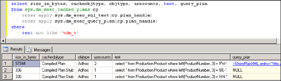
After executing sp_configure 'Optimize for ad hoc workloads', 1 and putting our database back into the simple parameterization mode, we reran our three queries from listing 17.4. After executing these queries, we inspected the procedure cache, the results of which are shown in figure 17.11.

Figure 17.11. After we enabled the Optimize for Ad Hoc Workloads option, ad hoc queries are stubbed and have no saved query plan.
 

There are a few things to point out here. First, note the cacheobjtype column for the three queries. Instead of Compiled Plan, we have Compiled Plan Stub. Second, note the size_in_bytes value (336 bytes vs. ~ 57,000/82,000 bytes in figure 17.9). Third, the join to the sys.dm_exec_query_plan function reveals the absence of a stored query plan.

What's happening here is that SQL Server detects these queries as ad hoc and not parameterized and therefore does not store a plan; however, it stores the stub in order to detect subsequent executions of the queries. For example, let's reexecute the first query from listing 17.4 and take another look at the procedure cache. The results are shown in figure 17.12.

Note the difference in the size_in_bytes, cacheobjtype, usecounts, and query_plan columns for the first query that we reexecuted. By saving the stub from the first execution, SQL Server is able to detect subsequent executions as duplicates of the first. Thus, it upgrades the plan from a stub to a full plan on the second execution, with the third (and subsequent) executions able to reuse the saved plan.

For environments containing large amounts of single-use ad hoc SQL, the Optimize for Ad Hoc Workloads option is a very significant new feature. Not only does it dramatically reduce the size of the procedure cache, but it still enables plan reuse in cases where identical ad hoc queries are executed many times, therefore also reducing CPU-related compilation pressure.

In closing our section on procedure cache usage, let's look at a number of techniques for measuring the cache contents and plan reuse.

Measuring procedure cache usage

The T-SQL code in listing 17.5 summarizes the contents of the sys.dm_exec_ cached_plans DMV. It lists the number of plans for each object type (ad hoc, prepared, proc, and so forth) along with the number of megabytes consumed by such plans and the average plan reuse count.

Example 17.5. Summary of procedure cache

-- Summary of Procedure Cache Contents
    SELECT
        objtype as [Object Type]
        , count(*) as [Plan Count]

Figure 17.12. Rerunning an ad hoc query converts the stub into a full plan.
 

, sum(cast(size_in_bytes as bigint))/1024/1024 as [Total Size (mb)]
        , avg(usecounts) as [Avg. Use Count]
    FROM sys.dm_exec_cached_plans
    GROUP BY objtype

Procedure caches suffering from a high volume of ad hoc SQL typically have a disproportionate volume of ad hoc/prepared plans with a low average use count. Listing 17.6 determines the size in megabytes of such queries with a single-use count.

Example 17.6. Size of single-use ad hoc plans

-- Procedure Cache space consumed by AhHoc Plans
    SELECT SUM(CAST(size_in_bytes AS bigint))/1024/1024 AS
         [Size of single use adhoc sql plans]
    FROM sys.dm_exec_cached_plans
    WHERE
        objtype IN ('Prepared', 'Adhoc')
        AND usecounts = 1

From a waits perspective, the RESOURCE_SEMAPHORE_QUERY_COMPILE wait type is a good indication of the presence of query compilation pressure. SQL Server 2005 introduced a throttling limit to the number of concurrent query compilations that can occur at any given moment. By doing so, it avoids situations where a sudden (and large) amount of memory is consumed for compilation purposes. A high incidence of this wait type may indicate that query plans are not being reused, a common problem with frequently executed unparameterized SQL.

Another method for determining plan reuse is measuring the following Performance Monitor counters:

• SQL Server SQL Statistics:SQL Compilations/Sec

• SQL Server SQL Statistics:SQL Re-Compilations/Sec

• SQL Server SQL Statistics:Batch Requests/Sec

With these counter values, we can measure plan reuse as follows:

Initial Compilations = SQL Compilations/Sec - SQL Recompilation/Sec
Plan Reuse = (Batch Req/sec - Initial Compilations) / Batch Req/sec

In other words, of the batch requests coming in per second, how many of them are resulting in query compilations? Ideally, in an OLTP system, this should be less than 10 percent, that is, a 90 percent or greater plan reuse. A value significantly less than this may indicate a high degree of compilations, and when observed in conjunction with significant RESOURCE_SEMAPHORE_QUERY_COMPILE waits, it's a reasonable sign that query parameterization may well be an issue, resulting in higher CPU and memory consumption.

Poor plan reuse not only has a direct impact on available RAM, but it also affects CPU usage courtesy of higher amounts of compilations. In the next section, we'll address CPU pressure from a general perspective.

17.3.2. CPU pressure

How do you measure CPU pressure for a SQL Server system? While classic Performance Monitor counters such as Processor:% Processor Time and System:Processor Queue Length provide a general overview, they are insufficient on their own to use in forming the correct conclusion. For that, we need to look a little further, with signal waits a critical consideration.

Signal waits

Earlier in the chapter, we looked at how SQLOS uses schedulers (figure 17.2) in allocating CPU time with processes (SPIDs) moving between three states: running, suspended, and runnable. There can be only a single SPID in the running status of a given scheduler at any one time, with the runnable queue containing SPIDs that are ready to run. The classic analogy used when discussing this model is the supermarket checkout line; that is, SPIDs in the runnable queue can be considered in the same manner as people lining up in the checkout queue: they have their groceries and are ready to leave, pending the availability of the checkout operator.

As we saw earlier, the sys.dm_os_wait_stats DMV includes a signal_wait_time_ms column, which indicates the amount of time, in total, processes spent in the runnable status for each wait type. Calculating the sum total of the signal wait time for all wait types as a percentage of the overall wait time gives a good indication of the depth of the runnable queue and therefore an indication of CPU pressure, from a SQL Server perspective.

When calculating the signal wait percentage, you should consider excluding certain wait types, LAZYWRITER_SLEEP, for example. Earlier in the chapter, we looked at the get/track_waitstats procedures, which take care of this automatically. A similar script is included toward the end of this section, in listing 17.7.

Generally speaking, a signal wait percentage of more than 25 percent may indicate CPU pressure, particularly in combination with a sustained high value for Processor:% Processor Time (> 80 percent). However, in some cases, CPU percentage may be well below 100 percent even though there is still significant CPU pressure. In such cases, the SOS_SCHEDULER_YIELD wait type is more than likely in the mix.

SOS_SCHEDULER_YIELD

As we covered earlier, a single SQLOS scheduler is created for each CPU core that a SQL Server instance has access to. When a request is sent to SQL Server for execution, it's assigned to a scheduler for execution and remains on that scheduler until complete. Despite SQL Server using various mechanisms for balancing load across the available schedulers, various situations may lead to a disproportionate load being assigned to a single scheduler.

Consider the following example: at a given point, all schedulers are equally busy, and two large CPU bound queries are submitted for execution. If they land on the same scheduler, they must remain on that scheduler until complete, even if load drops off the others. When multiple CPU bound tasks are executing on one scheduler, they yield to each other in order to ensure each task receives equal amounts of CPU time. In our example, the two large CPU bound tasks would be yielding to each other, despite the availability of a number of idle schedulers.^[] In this case, the total CPU percentage (as reported by Performance Monitor) may be well below 100 percent, even though there is significant contention on some CPU cores.

^[] In this case restarting one of the processes would more than likely position it on an idle scheduler.

Of course, if a system is completely CPU bound (all CPU cores), then the yielding process, exposed with the SOS_SCHEDULER_YIELD wait type, would be occurring on all schedulers. The important point is that the yielding process may be occurring on only some schedulers, even when overall CPU usage appears low. This makes the SOS_SCHEDULER_YIELD wait type an important consideration in an overall assessment of CPU pressure.

In closing this section on CPU pressure, let's look at some DMV queries that can be used in supplementing information from the waits and queues analysis.

DMV queries

The two DMV queries in this section identify signal wait percentage and top CPU consumers.

Listing 17.7 can be used to detect signal waits and resource waits as a percentage of the total wait time. As discussed previously, a high signal wait time usually indicates CPU pressure.

Example 17.7. Signal wait time

-- Wait Analysis; Signal vs. Resource Waits
SELECT
   SUM(wait_time_ms - signal_wait_time_ms) as [ResourceWaitTotal]
   , CAST(100.0 * sum(wait_time_ms - signal_wait_time_ms)
      / SUM(wait_time_ms) as numeric(20, 2)) AS [ResourceWait%]
   , SUM(signal_wait_time_ms) AS [SignalWaitTotal]
   , CAST (100.0 * sum(signal_wait_time_ms)
      / SUM (wait_time_ms) AS numeric(20, 2)) AS [SignalWait%]
FROM sys.dm_os_wait_stats
WHERE
    wait_type not in (
        'CLR_SEMAPHORE'
        , 'LAZYWRITER_SLEEP'
        , 'RESOURCE_QUEUE'
        , 'SLEEP_TASK'

, 'SLEEP_SYSTEMTASK'
        , 'WAITFOR'
    )

Notice that the script excludes a number of wait types not relevant to a performance-tuning process. The get/track_waitstats stored procedures we covered earlier perform the same exclusions.

Listing 17.8 lists the top 50 queries ordered by CPU time. It includes the execution_count column to indicate how many times this query has been executed. Frequently executed queries with large CPU consumption are targets for optimization.

Example 17.8. Top 50 queries by CPU consumption

-- Top 50 Queries by CPU Consumption
SELECT TOP 50
   queryStats.total_worker_time/queryStats.execution_count AS [Avg CPU
     
 Time]
   , queryStats.execution_count
   , SUBSTRING(queryText.text,queryStats.statement_start_offset/2,
     (CASE WHEN queryStats.statement_end_offset = -1
       THEN len(convert(nvarchar(max), queryText.text)) * 2
       ELSE queryStats.statement_end_offset end -
             queryStats.statement_start_offset) / 2)
AS query_text
    , dbname=db_name(queryText.dbid)
FROM sys.dm_exec_query_stats queryStats
   CROSS APPLY sys.dm_exec_sql_text(queryStats.sql_handle) AS queryText
ORDER BY
   [Avg CPU Time] DESC

One of the things that will become obvious as we move throughout this section is that common design problems affect a number of resources. For example, poor index selection and maintenance can have a dramatic impact on both memory and disk I/O.

17.3.3. Index-related memory pressure

As we covered in chapter 13, the correct selection and maintenance of indexes are crucial from a query-performance perspective. Numerous unused indexes have a large maintenance overhead, and missing or poorly maintained indexes have a double impact on resources: additional disk I/O and a reduction in the available buffer cache.

From a performance-monitoring perspective, the following performance counters are of interest in assessing the impact of poor index design and maintenance:

• SQL Server:Buffer Manager - Page Life Expectancy—This counter indicates the average time (in seconds) that data pages remain in memory. A common occurrence is for this value to drop suddenly in response to a large query that requires a lot of disk access, flushing data pages from memory to make way for the required data from disk. Missing indexes are a common contributor to this type of event. A system with adequate memory and good indexing should see this value in excess of 500 seconds, without frequent sudden drops during normal activity.

• SQL Server:Buffer Manager - Buffer Cache Hit Ratio—This counter indicates the percentage of time required pages are found in the buffer cache. The higher the value, the better, as memory access is obviously much faster than disk access. Once a SQL instance has been up and running for a period of time covering typical activity, values lower than 95 percent indicate memory pressure, one cause of which may be additional disk I/O required to fulfill queries without the appropriate indexes.

• SQL Server:Access Methods - Full Scans/Sec—This counter represents the number of full table (or index) scans per second. There are no benchmark numbers to compare this value against. In some cases, a table (or index) scan is actually preferred over an index lookup, as we discussed in chapter 13; however, one thing to look out for here is a sudden increase in this value, possibly indicating that an index is no longer being used. As with many other counters, baseline analysis is critical in being able to accurately detect a significant increase/decrease.

• SQL Server:Access Methods - Index Searches/Sec—Similar to Full Scans/Sec (but in the opposite direction), sudden decreases in this value may indicate an index is no longer being used.

• SQL Server:Access Methods - Page Splits/Sec—When a record is inserted into an index, it must be inserted in order. If the data page is full, the page splits in order to maintain the appropriate order. A high value for this counter may warrant the consideration of a lower fill factor, as covered in chapter 13.

In chapter 13, we covered a number of DMV-related queries that can be used to detect missing, unused, and duplicate/overlapping indexes. We won't duplicate coverage here.

In addition to increased memory pressure, poor index selection and maintenance have a direct and measurable impact on disk I/O.

17.3.4. Disk bottlenecks

Throughout this book we've covered a number of best practices pertaining to the layout of data and transaction log files, tempdb configuration, and sizing files to avoid autogrow operations. We've also covered the importance of striping data across multiple disks (spindles) and using RAID volumes for both performance and redundancy. With these things in mind, let's explore the waits and queues of significance in a disk bottleneck.

Waits

A classic performance-tuning dictum is there will always be a bottleneck somewhere, the idea being to address/reduce each bottleneck until performance is acceptable. As the slowest component, the bottleneck is usually on disk, on both high- and low-performing systems. The following wait types usually occupy the top two wait-list positions (after excluding system background waits) on systems experiencing disk bottlenecks:

• PAGEIOLATCH—As pages are read into the buffer cache from disk, SQL Server uses a series of latches (lightweight locks) on the buffer pages as they are filled with data and released to the requesting process. Both PAGEIOLATCH_SH and PAGEIOLATCH_EX are used as part of this process, and the appearance of these wait types in the top wait positions may be an indication of a disk I/O bottleneck, particularly when seen in combination with high disk sec/transfer counters, which we'll cover shortly.

• ASYNC/IO_COMPLETION—Both ASYNC_IO_COMPLETION and IO_COMPLETION indicate waits on disk I/O, with the async version typically associated with operations such as backups and restores.

• WRITELOG—This wait type is associated with writes to the transaction log. As covered throughout this book, locating transaction logs on dedicated disk volumes, preferably with a large battery-backed write cache, is essential in any high-volume database solution.

A top ranking of these waits necessitates the inspection of a number of related queues.

Queues

The classic disk-related Performance Monitor counters are PhysicalDisk:Avg. Disk Sec/Read and PhysicalDisk:Avg. Disk Sec/Write, with the commonly accepted ranges for performance as follows:

• < 10ms—Good

• 10-20ms—Average/typical performance

• 20-50ms—Slow

• > 50ms—Very slow, needs immediate attention

These counters measure the time in milliseconds for a read or write operation to disk and should be measured for each of the applicable disk volumes. For high-throughput applications, you need to pay particular attention to these counters for the transaction log disk, which should be well under 10ms.

As we covered earlier in the book, you should use the SQLIO and SQLIOSIM tools before commissioning any SQL Server system for production use to verify both the throughput and validity of the I/O system and compare the results to published vendor performance expectations. In addition to these counters, additional counters of interest are as follows:

• Physical Disk:% Disk Time—This counter measures the percentage of time the disk was busy servicing reads and writes. The generally accepted idea is that more than 50 percent may represent a bottleneck for the measured disk.

• Physical Disk:Avg./Current Disk Queue Length—A sustained value of more than 2 indicates the disk is struggling to service its queue. When measuring these counters, you need to consider the number of disks in the array. For example, a volume with 10 disks could reasonably service a queue of up to 20.

• Physical Disk:Avg. Disk Reads & Writes /Sec—As with the disk queue-length counters, you need to measure these counters in awareness of the disk volume's underlying disk count. Values approaching 90 percent of the disk's published read/writes per second capacity may indicate an approaching bottleneck.

Bear in mind that during disk-bound operations such as backups and restores, it's perfectly normal and reasonable to see sustained disk activity, with cause for concern centered on the speed or duration of the operation. For example, backing up a terabyte database to disk will obviously bottleneck on disk; however, the performance can be maximized by using dedicated backup disks, multiple backup files, and so forth.

In closing our brief look at disk I/O, let's examine a couple of DMV queries.

DMV queries

The two DMV queries in this section identify queries with the largest I/O usage and database files with the highest stall rates.

Listing 17.9 lists the top 50 queries ordered by I/O usage.

Example 17.9. Top 50 queries by I/O usage

-- Top 50 Queries by I/O Consumption
SELECT TOP 50
   (total_logical_reads + total_logical_writes) / execution_count AS [Avg
     
 IO]
   , substring (qt.text,qs.statement_start_offset/2, (
       CASE WHEN qs.statement_end_offset = -1
       THEN len(convert(nvarchar(max), qt.text)) * 2
       ELSE qs.statement_end_offset end - qs.statement_start_offset)/2
   ) AS query_text
   , qt.dbid
   , qt.objectid
FROM sys.dm_exec_query_stats qs
   CROSS APPLY sys.dm_exec_sql_text (qs.sql_handle) AS qt
ORDER BY [Avg IO] DESC

Listing 17.10 uses the sys.dm_io_virtual_file_stats function to inspect the stall rate of disk I/O per file. A stall occurs when a process waits for I/O to complete. By determining which files are stalling the most, opportunities arise for rebalancing I/O. A good example of this is multiple high-transaction-rate databases using the same physical disk(s). By segregating their database files on separate disks, you should be able to improve the throughput (and reduce the stall rate).

Example 17.10. Database file I/O stalls

-- Identify database files with the highest stall rate
SELECT
    db_name(database_id)
    , file_id
    , io_stall_read_ms
    , num_of_reads
    , cast(io_stall_read_ms/(1.0+num_of_reads) as numeric(10,1)) as
      'avg_read_stall_ms'
    , io_stall_write_ms
    , num_of_writes
    , cast(io_stall_write_ms/(1.0+num_of_writes) as numeric(10,1)) as
      'avg_write_stall_ms'
    , io_stall_read_ms + io_stall_write_ms as io_stalls

, num_of_reads + num_of_writes as total_io
    , cast((io_stall_read_ms+io_stall_write_ms)/(1.0+num_of_reads +
      num_of_writes) as numeric(10,1)) as 'avg_io_stall_ms'
FROM sys.dm_io_virtual_file_stats(null,null)
WHERE database_id > 4
ORDER BY
     database_id, avg_io_stall_ms DESC

As we covered in chapter 14, the Data File I/O pane in the new Activity Monitor presents some of this information in graphical form.

In closing this section on common performance problems, let's turn our attention to blocking.

17.3.5. Blocking

A block occurs when one query wants to access data that is locked by another. Despite blocks and locks being normal, fundamental components of any relational database management system, they present a significant problem in poorly designed databases and transactions.

In chapter 14, we covered the use of SQL Server Profiler in determining the presence of deadlocks and blocks exceeding a particular threshold. In this section, we'll cover blocking from a waits perspective.

LCK_* waits

SQL Server Books Online lists all of the wait types that may be encountered, including an impressive collection beginning with LCK_. All of these represent a wait on a particular lock being released. For example, a transaction with a shared lock on a row will block a separate transaction that requires an exclusive lock on the same row. In this case, the registered wait type will be LCK_M_X.

When the volume of locks and subsequent blocks increases, overall transaction throughput decreases, often accompanied by a reduction in Performance Monitor counters such as SQL Server SQL Statistics:Batch Requests/Sec. To the untrained eye, a severe blocking problem is often met with confusion; users complain of poor performance, but a quick check of the classic Performance Monitor counters (CPU, disk, and so forth) reveals little in the way of server load. When the blocking transaction completes, activity returns to normal.

A fundamental component of a good database design is short transaction length with the appropriate isolation level (and usually with an optimistic locking mode). Such topics are beyond the scope of this book: however, should you identify blocking as a top wait type, the sys.dm_db_index_operational_stats function can assist you in investigating the problem further.

sys.sm_db_index_operational_stats

One of the purposes of the sys.dm_db_index_operational_stats function is to determine the tables and indexes with the highest occurrence of row lock waits, as shown in listing 17.11.

Example 17.11. Tables/indexes with high lock waits

— Identify tables and indexes with the highest number of row lock waits
SELECT
   db_name(db_id())
   , object_name(s.object_id) as objectname
   , i.name as indexname
   , row_lock_count
   , row_lock_wait_count
   , cast (100.0 * row_lock_wait_count /
     (1 + row_lock_count) as numeric(15,2)) as [block %]
   , row_lock_wait_in_ms
   , cast (1.0 * row_lock_wait_in_ms /
     (1 + row_lock_wait_count) as numeric(15,2)) as [avg row lock waits in
         
 ms]
FROM sys.dm_db_index_operational_stats (db_id(), NULL, NULL, NULL) s
   INNER JOIN sys.indexes i on s.object_id = i.object_id
   AND s.index_id = i.index_id
WHERE objectproperty(s.object_id,'IsUserTable') = 1
ORDER BY row_lock_wait_count desc

In combination with the SQL Profiler blocked process report event, this script can be used to identify the source of common blocking problems. The avg row lock waits in ms column, as the name suggests, returns the average lock wait time. This value can be used in estimating which value to set for the sp_configure 'blocked process threshold' value, although it should be noted that the sp_configure value is set in seconds, whereas the value returned from the above script is in milliseconds.

In closing the chapter, let's summarize the waits, queues, and DMV scripts that we've covered thus far into resource categories.