
14.2. SQL Server Profiler
Prior to SQL Server 2005 (and the introduction of DMVs), SQL Server Profiler was one of the few tools that could be used to gain visibility of SQL Server activity and was therefore used for a broad range of performance and debugging purposes. As you'll soon see, Profiler remains an extremely versatile tool; however, it's often used for the wrong reasons, creating significant performance problems as a result.
In chapter 17 we'll introduce a performance-tuning methodology called waits and queues, which uses a combination of DMVs and Performance Monitor counters to narrow the scope of a performance-tuning exercise by focusing on the largest system bottlenecks. Such an approach is far more effective than a Profiler-only approach, frequently used in years gone by and still used by some.
In this section, we'll focus on using Profiler for alternate purposes, namely workload replay and deadlocked/blocked process analysis. We'll also cover the important difference between a Profiler trace and a server trace. Before we get to that, let's begin with perhaps the most common use for Profiler: workload analysis.
14.2.1. Workload analysis
A common task in a performance-tuning exercise is analyzing the cost of the queries that make up an application's workload. For example, if CPU is a significant system bottleneck, you need to establish which queries consume the most CPU. Profiler enables such analysis through its ability to capture, or trace, the execution of queries along with their associated cost metrics, that is, disk reads and writes, CPU usage, and duration.
As we've just explained, using Profiler as the only performance-tuning tool ignores much more effective options; however, for the purposes of introducing Profiler, let's proceed on that basis with a simple example.
SQL Server Profiler can be accessed through the Performance Tools folder of the SQL Server program group. After opening Profiler and choosing File > New Trace, you're prompted with the Connect to Server dialog box, which enables you to select a SQL instance to trace. After connecting to an instance, you're presented with the Trace Properties window, as shown in figure 14.5.
Figure 14.5. The General Tab of a Profiler Trace Properties window enables us to select the trace location along with a template and stop time.
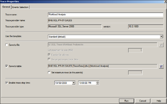
After giving the trace a name, you can choose to base the trace on a template, which is used to define the included columns and events on the Events Selection tab, which we'll cover shortly. By default, the output of the trace is displayed to screen only. For this example, we'll choose to save the results to a table for reasons that will become apparent shortly.
After entering an optional stop time (a trace can also be manually stopped), click the Events Selection tab, as shown in figure 14.6, to choose the included events and event columns.
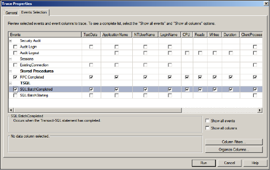
For the purposes of this example, we'll limit the included events to the RPC:Completed and SQL:BatchCompleted events. These events represent the completion of T-SQL batches and stored procedures and include the associated cost metrics. The Column Filters button enables us to apply filters, such as limiting the trace to include events for a particular user or database, or queries exceeding a particular duration or cost. As mentioned earlier, when we launch SQL Profiler via the Activity Monitor's Processors pane, a filter is automatically applied for the selected SPID.
Finally, selecting the Show All Events and Show All Columns check boxes enables the inclusion of additional events and columns from the full list, rather than the limited set derived from the selected template on the General tab.
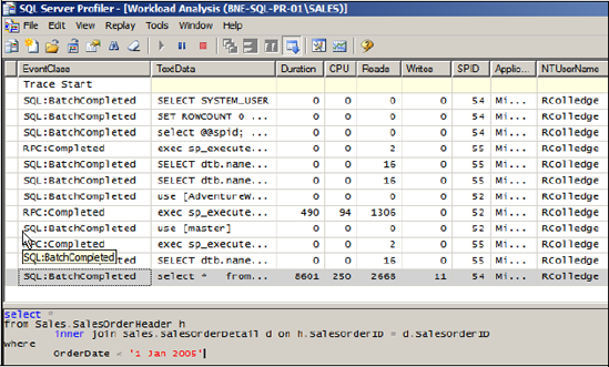
Once you're ready, click Run, and the trace begins and database activity matching the selected events and filters is displayed on screen. For this example, a small number of queries were executed in Management Studio after the trace was started, the result of which is shown in figure 14.7.
Figure 14.6. The Events Selection tab enables the selection of events and columns for inclusion in the trace results.
A quick inspection of the Profiler trace screen reveals that the values of the Duration, CPU, and Reads columns for the last row are clearly greater than the rest of the captured values. Clicking on this record displays the query text in the lower section of the Profiler window.
For a simple example such as this, you can visually browse the small number of captured events. However, when a real trace is run and captured over a period of time representing peak production activity, the number of captured events typically runs into the thousands (or more). Not only does this prevent a visual analysis of activity, but it can also cause significant performance problems. In addressing this, you can use a server-side trace.
Figure 14.7. The output of a Profiler trace is shown on screen as well as saved to file and table if these options were chosen.
14.2.2. Server-side trace
Using SQL Server Profiler to trace database activity is frequently referred to as client-side tracing, that is, events are streamed from the server, over the network, to the Profiler application. Even if the Profiler application is being run on the SQL Server itself, this is still considered a client-side trace.
One of the worrisome aspects of client-side tracing with SQL Profiler is that under certain conditions, events can be dropped, therefore invalidating event sequencing and performance analysis. Further, depending on the server load, the overhead of streaming events can impact server performance, in some cases quite dramatically.
SQL Server Profiler is a GUI-based client interface to SQL Trace, the event-tracing service within the database engine. As an alternative to using SQL Profiler, we can create a server-side trace using a number of SQL Trace system stored procedures and in doing so avoid both the performance problems and dropped events commonly associated with client-side traces.
A good example of a server-side trace is the SQL Server default trace, a lightweight, always-on trace recording selected events, primarily configuration changes. As shown in figure 14.8, the Configuration Changes History standard report, accessed by right-clicking a server instance and choosing Reports, uses this trace to display the date and time of recent configuration changes. The log files created by this trace (named log_1.trc, log_2.trc, and so forth) are stored in the default MSSQLLOG directory and can be opened in SQL Profiler for inspection if required.
As we said earlier, one of the nice things about SQL Profiler is the ease with which a trace can be created and executed, particularly when compared to the alternative of creating T-SQL scripts using the SQL Trace procedures. Fortunately, one of the options available within SQL Profiler is the ability to script a trace definition, which can then be used in creating a server-side trace. Creating a trace in this manner, we get the best of both worlds: using the Profiler GUI to create our traces, yet running the trace as a server-side trace, thereby avoiding the performance overhead and dropped events associated with client-side traces.
Figure 14.8. One of the many available standard reports
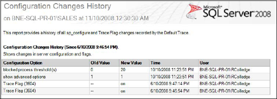
Figure 14.9. A Profiler trace can be scripted to file for execution as a server-side trace. Before doing so, we must specify the trace file location, as per the highlighted text.
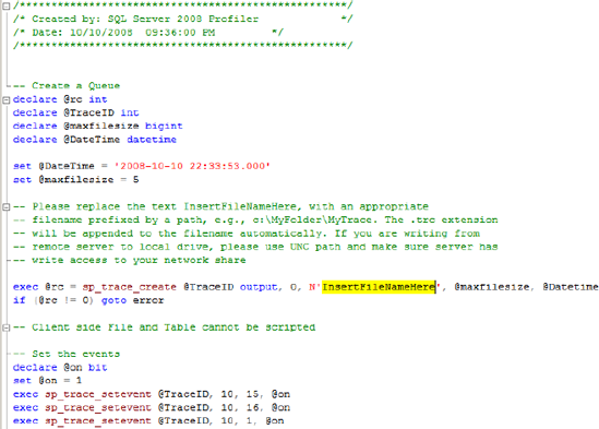
A Profiler trace can be exported to a file using the File > Export menu item after the trace has been defined with the required events, columns, and filters. The resultant T-SQL code, an example of which is shown in figure 14.9, can then be executed against the required instance, which creates the server-side trace. Once the trace is created, we can use the sp_trace_setstatus and fn_trace_getinfo commands, as documented in Books Online, to control and inspect the trace status.
As per figure 14.9, we specify the trace file location by editing the sp_trace_create parameters in the script produced by SQL Server Profiler.
One of the important aspects of a server-side trace is that events cannot be dropped; that is, system throughput may slow if writing the trace file becomes a bottleneck. While the overhead in writing a server-side trace file is significantly lower than the Profiler equivalent, it's an important consideration nonetheless. Therefore the trace file should be treated in a similar manner to a transaction log file, that is, located on a dedicated, high-speed disk that's local to the server instance—not a network file share.
With the importance of client-side versus server-side traces in mind, let's continue and look at a number of alternate uses for SQL Server Profiler, starting with the ability to replay a trace.
14.2.3. Trace replay
Trace replay refers to the process whereby a captured trace file is replayed against a database to regenerate the commands as they occurred when the trace was captured. Such a process is typically used for both debugging and load generation.
Capturing a trace that will be used for replay purposes requires particular events and columns to be included. The easiest way to do this is by using SQL Profiler's TSQL_Replay template when entering the details in the Trace Properties window, as shown earlier in figure 14.5. Selecting this template will ensure all of the necessary events and columns are included for replay.
When the trace has captured the required events, you can invoke replay by opening the trace file or table in SQL Profiler and selecting Start from the Replay menu. The resultant screen, as shown in figure 14.10, enables various options during replay.
Understanding the replay options is crucial in understanding some of the limitations of using it:
Replay Server allows the selection of the server instance where the trace file will be replayed. Notice there is no mention of which database to replay the trace against. The database with the same name (and database ID) should exist on the replay instance, which is usually an instance separate from where the trace was captured. If so, the replay instance should also include the same logins, passwords, users, and default databases applicable to the captured trace.
Save to File/Table enables the results of the replay to be captured to a file or table. The captured results include the full output of the replayed commands. For example, a select command that returns 10 rows will result in 10 rows in the trace replay output file/table. The resultant output can be potentially huge and should therefore be chosen with caution; however, used correctly, this option is invaluable for debugging purposes.
Number of Replay Threads enables the degree of concurrency to be set for replay purposes. A high number of threads will consume more resources but will result in a faster replay.
Replay Events in the Order They Were Traced will do exactly that and is the option to use when reconstructing an event for debugging purposes.
Figure 14.10. Trace replay options include saving results to file and/or table and controlling replay concurrency with multiple threads.
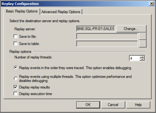
Replay Events Using Multiple Threads is the high-performance replay mode that disables debugging. Events are replayed using multiple threads, with each thread ordering events for a given SPID; for example, SPID 55 will have its events replayed in the correct order, but its events may be replayed before SPID 68, even though SPID 68's events occurred first.
Display Replay Results shows the results of the replay on screen. The same warnings apply here as for the Save to File/Table options we covered earlier.
For the purposes of debugging complex application problems, SQL Profiler's trace replay is undoubtedly a powerful tool, particularly when debugging in a live production environment is not an option. In such cases, a production database backup is typically restored in a testing environment followed by the replay of a trace captured while the problem was reproduced in production. Once captured, the trace can be replayed in a testing environment multiple times, optionally preceded by a database restore before each replay. Debug options such as Run to Cursor and Toggle Breakpoint enable classic debugging by replaying the trace to a certain point, inspecting the output, and then iteratively moving through the remaining events as required.
Despite its strengths, there are a number of limitations with trace replay that you need to understand. SQL Server Books Online documents all of them, but the major limitation is its lack of support for traces containing certain data types and activity; for example, a trace containing transactional replication, GUID operations, or Bulk Copy Process (BCP) actions on n/text or image columns cannot be replayed. Further, the logins and users referenced in the trace must exist on the target instance with the same permissions, passwords, default database, and database ID.
Another common use for replaying trace files is simulating load for change and/or configuration-testing purposes. Capturing a trace during a peak load period allows performance to be observed in a test environment under different configuration settings; however, despite the ability to increase the number of threads during playback, a trace replay cannot exactly reproduce the timing and sequencing of events as they occurred during the capture of the trace. Using the Replay Events in the Order They Were Traced option will guarantee event sequencing but will not simulate concurrent activity. Conversely, using Replay Events Using Multiple Threads will generate simultaneous event replay but at the expense of event sequencing across all SPIDs.
One of the things preventing exact event reproduction is the inability to use multiple replay machines, a limitation addressed in the RML utilities.
14.2.4. RML utilities
For many years, Microsoft Product Support Services (PSS) used a collection of private tools for assisting in the diagnosis and resolution of customer support issues. Now known as the replay markup language (RML) utilities, PSS released them to the general public in 2004.
Available as a free download from the Microsoft website, the RML utilities, comprising ReadTrace, Reporter, and OStress, are used both for diagnosing performance problems and constructing stress-test scenarios.
ReadTrace and Reporter
When we defined our Profiler trace earlier in figure 14.5, we chose to save the results to a database table. Doing so allows the results of the trace to be examined in a variety of ways once the trace is closed. For example, we could run the following query against the specified table to determine the top 10 expensive queries from a disk-usage perspective:
-- Top 10 most expensive queries from a disk usage perspective
SELECT TOP 10 TextData, CPU, (Reads + Writes) as DiskTotal, Duration
FROM dbo.[Workload Analysis]
ORDER BY DiskTotal DESC
Queries such as the above are among the many possible ways in which the results can be analyzed. Further, as we saw in chapter 13, we can use the saved results as input for the Database Engine Tuning Advisor, which will analyze the trace contents and make various recommendations.
One of the limitations of using Profiler for workload analysis such as this is that query executions that are the same with the exception of the literal values are difficult to analyze together as a group. Take these two queries, for example:
SELECT * FROM [authors] WHERE [lastName] = 'Smith'

SELECT * FROM "authors" WHERE "lastName" = 'Brown'
These are really different versions of the same query, so grouping them together for the purpose of obtaining the aggregate cost of the query is beneficial; however, without a significant amount of string-manipulation logic, this would be difficult to achieve. ReadTrace performs such grouping analysis automatically.
Executed at the command line with a number of input parameters including a trace file name, ReadTrace
Creates a new database, by default named PerfAnalysis, in a specified SQL Server instance
Analyzes and aggregates information contained within the trace file and stores the results in the PerfAnalysis database
Produces .RML files, which can be used as input for the OStress utility, which we'll discuss shortly
Launches the Reporter utility, which graphically summarizes the results captured in the PerfAnalysis database
The first step in using ReadTrace is capturing a trace file. In order for ReadTrace to work and provide the most beneficial analysis, we need to include a number of events and columns in the trace. The help file that's supplied with the RML utilities documents all the required events and columns.
Once the trace file has been captured, the ReadTrace utility can be executed against it, an example of which follows:
Readtrace -IG:TraceSalesTrace_1.trc -o"c:	emp
ml" -SBNE-SQL-PR-01SALES
Figure 14.11. Figure One of the many reports available in the RML Reporter utility. This one breaks down resource usage by query.

Once processing is complete, the Reporter utility automatically opens and displays the results of the analysis. The example report shown in figure 14.11 demonstrates one of the clear advantages of using the ReadTrace/Reporter utilities over manual analysis of SQL Profiler results stored in a table. Note the {STR} value in the Query Template column at the very bottom of the report for Query 1. The ReadTrace utility analyzes and aggregates different executions of the same query/stored procedure as a group by stripping out literal values such as stored procedure parameter values. In the example shown, {STR} represents RML's understanding of this as a parameter value. Thus, the total cost of all executions of this stored procedure will be automatically calculated.
In addition to viewing the results of ReadTrace analysis via the Reporter utility, you can directly query the PerfAnalysis database for more advanced analysis.
Finally, one of the major benefits of ReadTrace is the .RML files it creates once processing is complete. The OStress utility can use these files for both replay and stress-testing purposes.
OStress
When covering the SQL Profiler trace replay option earlier in the chapter, we discussed one of its limitations: the inability to use multiple machines for replay purposes,thereby limiting the scale of the load that can be achieved. In contrast, OStress has no such limitation.
Like ReadTrace, OStress is a command-line utility. It's used to execute a command or series of commands against a supplied instance and database. Its input can be a single inline query, a query file, or an .RML file produced by the ReadTrace utility. Consider the following example:
ostress -o"c: empo" -SBNE-SQL-PR-01SALES -dOrders -iStress.sql -n10 -r25
The end result of running the above command will be to spawn 10 threads (-n parameter), each of which will execute the contents of the Stress.sql file against the Orders database 25 times (-r parameter), for a total of 250 executions. Further, this could potentially run on multiple machines simultaneously, each of which is stressing the same database. You can imagine the scale of stress that could be achieved!
The -i parameter also accepts RML files as input, and the -Q parameter is used for a single inline query. If an RML file is used, -m replay can be used to instruct OStress to use replay mode instead of stress mode. In replay mode, events are replayed in the sequence in which they were captured. In contrast, stress mode replays events as fast as possible for maximum stress.
In addition to load generation and debugging, SQL Server Profiler can also be used in diagnosing deadlocks.
14.2.5. Deadlock diagnosis
Troubleshooting deadlocks isn't the nicest (or easiest) task for a DBA; however, SQL Profiler makes it much simpler. In demonstrating this, consider listing 14.1, which contains a simple T-SQL batch file. When a second instance of this batch file is executed within 10 seconds of the first (from a separate connection/query window), a deadlock will occur, with the second query chosen as the deadlock victim and killed by SQL Server.
Example 14.1. T-SQL code to generate a deadlock
-- T-SQL to simulate a deadlock. Run this from 2 separate query windows
-- The 2nd will deadlock if executed within 10 seconds of the 1st

SET TRANSACTION ISOLATION LEVEL SERIALIZABLE -- hold share lock till end
BEGIN TRANSACTION
SELECT * FROM HumanResources.Department
WAITFOR DELAY '00:00:10.000' -- delay for 2nd transaction to start
UPDATE HumanResources.Department
SET Name = 'Production'
WHERE DepartmentID=7
COMMIT TRANSACTION |
What's happening here is that the shared lock on the HumanResources.Department table is being held until the end of the transaction, courtesy of the Serializable isolation level chosen at the start of the batch. When the update command runs later in the transaction, the locks need to be upgraded to an exclusive lock. However, in the meantime, another instance of this batch has run, which also has a shared lock on the HumanResources.Department table and also needs to upgrade its locks. Both transactions will wait on each other forever. SQL Server detects this situation as a deadlock and chooses to kill one of the transactions to enable the other to complete.
When creating a Profiler trace, one of the events we can capture is the deadlock graph, found under the Locks category when the Show All Events check box is checked. We saw this check box earlier in figure 14.6. When we select the deadlock event, an additional tab becomes available in the Trace Properties window, which enables the deadlock graph(s) to be saved to a file.
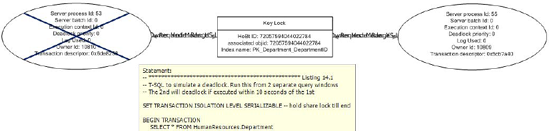
With this event selected and the trace running, executing the above code from two separate connections will generate a deadlock graph event and a deadlock results file. Opening the file in SQL Server Management Studio (by double-clicking it) will reveal the graph shown in figure 14.12.
You'll notice in the above image the blue X through the left-hand query. This was the chosen deadlock victim. Hovering the mouse over the query will reveal the query text. The item in the middle of the graph represents the resource that the two queries deadlocked over.
The ability to easily capture deadlock information using Profiler makes the process of identifying the application or database code causing the deadlocks significantly easier.
Figure 14.12. The deadlock graph event can be included in a trace to visually represent the deadlock, including details such as the deadlock victim and resource.
Not only can Profiler detect deadlocks, it can also be used to detect blocked processes.
14.2.6. Blocked process report
When a process attempts to lock a resource that's currently locked by another process, it waits for the lock to be released, and it's known for the duration of the wait as a blocked process. Unlike deadlocks, blocked processes are perfectly normal; however, depending on the frequency and duration of the waits, blocked processes can significantly contribute to poor application performance. Consider the code in listing 14.2.
Example 14.2. T-SQL code to generate a block
-- T-SQL to simulate lengthly locking period BEGIN TRANSACTION SELECT * FROM HumanResources.Department(xlock) WAITFOR DELAY '00:00:50.000' — hold lock for 50 seconds COMMIT TRANSACTION |
What we're doing here is simulating a long-running transaction that holds locks for the duration of the transaction, in this case an exclusive lock on the department table for 50 seconds. Similar to our deadlock example earlier, we'll run this batch from two separate connections. With the first execution holding an exclusive lock on the department table, the second execution will be blocked, waiting for the first to complete.
In helping to diagnose blocked processes such as the one that we're simulating here, we can set the Blocked Process Threshold server configuration setting. As shown listing 14.3, this setting takes a parameter representing the number of seconds a process can be blocked before an alert is raised. Let's configure this value to 20 seconds.
Example 14.3. Setting the Blocked Process Threshold
-- Set the Blocked Process Threshold to 20 seconds EXEC sp_configure 'show advanced options', 1 GO RECONFIGURE GO EXEC sp_configure 'blocked process threshold', 20 GO RECONFIGURE GO |
Figure 14.13. You can use the Blocked Process Report event in combination with the Blocked Process Threshold setting to capture blocking events exceeding a certain duration.
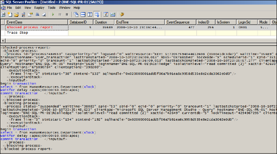
With this setting in place, we can create a SQL Server Profiler trace that profiles the Blocked Process Report event (found in the Errors and Warnings category). After running the T-SQL batch from two separate connections, our Profiler trace will capture the Blocked Process Report event, as shown in figure 14.13. The XML contained within the report provides details on both the blocking and blocked processes, including the T-SQL, client application, and login name.
A common characteristic of poorly designed database applications is frequent and lengthy process blocking, largely due to inappropriate locking levels and transaction length. In combination with the Blocked Process Threshold setting, SQL Server Profiler's Blocked Process Report event offers an effective and easily implemented method of detecting and analyzing such blocking events.
In closing our coverage of SQL Server Profiler, let's look at how we can enhance the collected events with Performance Monitor data.
14.2.7. Correlating traces with performance logs
Correlating different perspectives of the same event almost always leads to a deeper understanding of any situation. In SQL Server monitoring, one of the opportunities we have for doing that is importing Performance Monitor data into a Profiler trace, as shown in figure 14.14.
After opening a saved Profiler trace file (or table), you can choose the File > Import Performance Data menu option to select a Performance Monitor log file to import. You can then select the appropriate counters from the log for inclusion.
Figure 14.14. Profiler allows Performance Monitor logs to be imported, and this permits correlation of Profiler events with the corresponding Performance Monitor counters of interest.

Once the log file is imported, clicking a particular traced command in the top half of the window will move the red bar to the appropriate spot in the Performance Monitor log (and vice versa). In the example shown in figure 14.14, you can see a spike in CPU usage just over halfway through the displayed time frame. Clicking on the start of the spike will select the appropriate command in the trace results, with the full command shown at the bottom of the screen. In this example, you can see the cause of the CPU spike: a cross join between two tables with a random ordering clause.
In addition to enhancing our Profiler traces, Performance Monitor data is invaluable in gaining a deeper understanding of SQL Server activity, as well as enabling baseline analysis, both of which we'll cover next.