13.2. Index design

A good database design is made in conjunction with, and is conscious of, application data access logic. For example, in order to design indexes for a particular table, the database designer must know how users will be accessing the table from the application(s). If an application allows searching for data on a particular column or set of columns, then this needs to be considered from an indexing point of view. That's not to suggest that the application completely dictates index design. The reverse is often true; sometimes unrealistic application access must be modified in order to prevent user-generated activity that causes database performance problems.

In this section, we'll concentrate on generic index design strategies, beginning with the type of columns suitable for a clustered index. We'll then look at an area we touched on in our introduction, covering indexes and included columns, before concluding the section with coverage of a new feature in SQL Server 2008, filtered indexes, and how they compare with indexed views.

Let's begin with an important step in table design: selecting a clustered index.

13.2.1. Selecting a clustered index

When a table is created with a primary key constraint, as per the following example, a unique clustered index is automatically created on the column(s) in the primary key, unless specified otherwise.

-- Creates a clustered index by default on the clientCode primary key
CREATE TABLE dbo.client (
    clientCode int PRIMARY KEY
    , surname nvarchar(100)
    , firstName nvarchar(100)
    , SSN char(11)
    , DOB datetime
)
GO

In this example, the clientCode column will be used as the primary key of the table as well as the unique clustered index. Defining the column as the primary key means an explicit CREATE CLUSTERED INDEX command is not required. Should we wish to create the clustered index on a different column, SSN for example, we could create the table as follows:

-- Create a clustered index on a nonprimary key column
CREATE TABLE dbo.client (
    clientCode int PRIMARY KEY NONCLUSTERED
    , surname nvarchar(100)
    , firstName nvarchar(100)
    , SSN char(11)
    , DOB datetime
)
GO

CREATE UNIQUE CLUSTERED INDEX cixClientSSN ON dbo.client(SSN)
GO

Created in this manner, the client table will contain two indexes: a unique nonclustered index for the primary key constraint and a unique clustered index for the SSN column.

So, generally speaking, which types of columns make the best candidates for a clustered index? In answering this, let's recap some points from earlier in the chapter:

• The clustered index key is contained in the leaf node of each nonclustered index as the row locator. If the clustered index changes from one column to another, each nonclustered index needs to be updated in order to maintain the linkage from the nonclustered index to the base table. Further, if the column value of the clustered index changes, similar updates are required in each of the nonclustered indexes.

• The width of the clustered index directly affects the size of each nonclustered index. Again, this is a consequence of including the clustered index key in the leaf node of each nonclustered index.

• If a clustered index is not unique, SQL Server will make it so by adding a hidden uniqueifier column to the table for inclusion in the index.

It follows that the best candidates for a clustered index are columns that

• Change infrequently (ideally not at all)—A stable column value avoids the need to maintain nonclustered index row locators.

• Are narrow—They limit the size of each nonclustered index.

• Are unique—They avoid the need for a uniqueifier.

With these attributes in mind, a common pattern for table design is to create what's called a surrogate key, using the IDENTITY property as per this example:

-- Use the IDENTITY property to create a clustered primary key column
CREATE TABLE dbo.client (
    clientKey int IDENTITY (1,1) PRIMARY KEY
    , surname nvarchar(100)
    , firstName nvarchar(100)
    , SSN char(11)
    , DOB datetime
)
GO

By adding the IDENTITY (1,1) property to the clientKey column definition, SQL Server will populate this column's value with an automatically incrementing number for each new row, starting at 1 for the first row and increasing upward by 1 for each new row.

Using the IDENTITY property to create a surrogate key in this manner meets the desired attributes for a clustered index. It's an arbitrary number used purely to identify the record, and therefore it has no reason to be modified. It's narrow: a single integer-based column will occupy only 4 bytes. Finally, it's unique; SQL Server will automatically take care of the uniqueness, courtesy of the IDENTITY property.

In our client table example, the other candidate for a clustered index, as well as the primary key, is the Social Security number. It's reasonably narrow (11 bytes), unlikely to change, and unique. In fact, if we made SSN the unique clustered primary key, we'd have no need for the identity-based clientKey column. But there's one big problem here. It's unique for those who have an SSN. What about those who don't have one or those who can't recall it? If the SSN was the primary key value, the lack of an SSN would prevent a row from being inserted into the table.^[] For this reason, the best primary keys/unique clustered indexes tend to be artificial or surrogate keys that lack meaning and use system-generated uniqueness features such as the identity column. Of course, there are exceptions to this rule, and this is a commonly argued point among database design professionals.

^[] As an Australian without a U.S. Social Security number, I've witnessed this firsthand.

The other consideration for a clustered index is column(s) involved in frequent range scans and queries that require sorted data.

Range scans and sort operations

Earlier in the chapter we covered the case where nonclustered indexes are sometimes ignored if the estimated number of rows to be returned exceeds a certain percentage. The reason for this is the accumulated cost of the individual key/RID lookup and random I/O operations for each row.

For tables that are frequently used in range-scanning operations, clustering on the column(s) used in the range scan can provide a big performance boost. As an example, consider a sales table with an orderDate column and frequent queries such as this one:

-- Range Scan - Potential for a clustered index on orderDate?
SELECT *
FROM dbo.sales
WHERE orderDate BETWEEN '1 Jan 2008' AND '1 Feb 2008'

Depending on the statistics, a nonclustered index seek on orderDate will more than likely be ignored because of the number of key lookups involved. However, a clustered index on orderDate would be ideal; using the clustered index, SQL Server would quickly locate the first order and then use sequential I/O to return all remaining orders for the date range.

Finally, queries that select large volumes of sorted (ORDER BY) data often benefit from clustered indexes on the column used in the ORDER BY clause. With the data already sorted in the clustered index, the sort operation is avoided, boosting performance.

Often, a number of attributes come together to make a column an ideal clustered index candidate. Take, for example, the previous query, which selects orders based on a date range; if that query also required orders to be sorted, then we could avoid both key lookups and sort operations by clustering on orderDate.

As with most recommendations throughout this book, the process for choosing the best clustered index is obviously dependent on the specifics of each database table and knowledge of how applications use the table. That being said, the above recommendations hold true in most cases. In a similar manner, there are a number of common techniques used in designing nonclustered indexes.

13.2.2. Improving nonclustered index efficiency

As we've covered throughout this chapter, the accumulated cost of random I/O involved in key/RID lookups often leads to nonclustered indexes being ignored in favor of sequential I/O with clustered index scans. To illustrate this and explore options for avoiding the key lookup process, let's walk through a number of examples using the Person. Contact table in the sample AdventureWorks database. In demonstrating how SQL Server uses different indexes for different queries, we'll view the graphical execution plans, which use different icons, as shown in figure 13.4, to represent different actions (lookups, scans, seeks, and so forth).

Figure 13.4. Common icons used in graphical execution plans
 

The Person.Contact table, as defined below (abbreviated table definition), contains approximately 20,000 rows. For the purposes of this test, we'll create a nonunique, nonclustered index on the LastName column:

-- Create a contact table with a nonclustered index on LastName
CREATE TABLE [Person].[Contact](
   [ContactID] [int] IDENTITY(1,1) PRIMARY KEY CLUSTERED
   , [Title] [nvarchar](8) NULL
   , [FirstName] [dbo].[Name] NOT NULL
   , [LastName] [dbo].[Name] NOT NULL
   , [EmailAddress] [nvarchar](50) NULL
)
GO

CREATE NONCLUSTERED INDEX [ixContactLastName] ON [Person].[Contact]
   ([LastName] ASC)

GO

For our first example, let's run a query to return all contacts with a LastName starting with C:

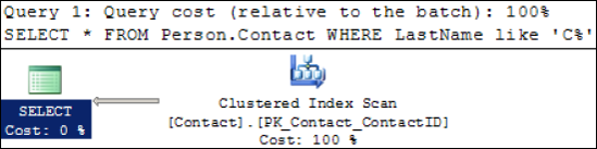
-- Statistics indicate too many rows for an index lookup
SELECT *
FROM Person.Contact
WHERE LastName like 'C%'

Despite the presence of a nonclustered index on LastName, which in theory could be used for this query, SQL Server correctly ignores it in favor of a clustered index scan. If we execute this query in SQL Server Management Studio using the Include Actual Execution Plan option (Ctrl+M, or select from the Query menu), we can see the graphical representation of the query execution, as shown in figure 13.5.

Figure 13.5. A clustered index scan is favored for this query in place of a nonclustered index seek plus key lookup.
 

No great surprises here; SQL Server is performing a clustered index scan to retrieve the results. Using an index hint, let's rerun this query and force SQL Server to use the ixContactLastName index:

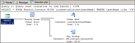
-- Force the index lookup with an index hint
SELECT *
FROM Person.Contact WITH (index=ixContactLastName)
WHERE LastName like 'C%'

Looking at the graphical execution plan, we can confirm that the index is being used, as per figure 13.6.

Figure 13.6. Adding an index hint to the previous query results in an index seek plus key lookup.
 

On a small database such as AdventureWorks, the performance difference between these two methods is negligible; both complete in under a second. To better understand how much slower the index lookup method is, we can use the SET STATISTICS IO option, which returns disk usage statistics^[] alongside the query results. Consider the script in listing 13.2.

^[] Not to be confused with index statistics, query statistics refer to disk usage, such as the number of pages read from buffer or physical disk reads.

Example 13.2. Comparing query execution methods

-- Compare the Disk I/O with and without an index lookup
SET STATISTICS IO ON
GO

DBCC DROPCLEANBUFFERS
GO

SELECT *
FROM Person.Contact
WHERE LastName like 'C%'

DBCC DROPCLEANBUFFERS

SELECT *
FROM Person.Contact with (index=ixContactLastName)
WHERE LastName like 'C%'
GO

This script will run the query with and without the index hint. Before each query, we'll clear the buffer cache using DBCC DROPCLEANBUFFERS to eliminate the memory cache effects. The STATISTICS IO option will produce, for each query, the number of logical, physical, and read-ahead pages, defined as follows:

• Logical Reads—Represents the number of pages read from the data cache.

• Physical Reads—If the required page is not in cache, it will be read from disk. It follows that this value will be the same or less than the Logical Reads counter.

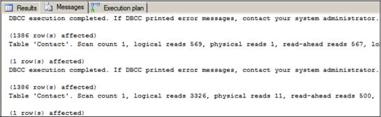
  Figure 13.7. Forcing a nonclustered index seek plus key lookup significantly increases the number of pages read.
   

  

• Read Ahead Reads—The SQL Server storage engine uses a performance optimization technique called Read Ahead, which anticipates a query's future page needs and prefetches those pages from disk into the data cache. In doing so, the pages are available in cache when required, avoiding the need for the query to wait on future physical page reads.

So with these definitions in mind, let's look at the STATISTICS IO output in figure 13.7.

These statistics make for some very interesting reading. Note the big increase in logical reads (3326 versus 569) for the second query, which contains the (index= ixContactLastName) hint. Why such a big increase? A quick check of sys.dm_ db_index_physical_stats, covered in more detail later in the chapter, reveals there are only 570 pages in the table/clustered index. This is consistent with the statistics from the query that used the clustered index scan. So how can the query using the nonclustered index read so many more pages? The answer lies in the key lookup.

What's actually occurring here is that a number of clustered index pages are being read more than once. In addition to reading the nonclustered index pages for matching records, each key lookup reads pages from the clustered index to compete the query. In this case, a number of the key lookups are rereading the same clustered index page. Clearly a single clustered index scan is more efficient, and SQL Server was right to ignore the nonclustered index.

Let's move on to look at an example where SQL Server uses the nonclustered index without any index hints:

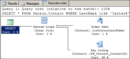
SELECT *
FROM Person.Contact
WHERE LastName like 'Carter%'

The graphical execution plan for this query is shown in figure 13.8, and it confirms the index is being used.

We can see that of the overall query cost, 98 percent is the key lookup. Eliminating this step will derive a further performance increase. You'll note that in our queries so far we've been using select *; what if we reduced the required columns for the query to only those actually required and included them in the index? Such an index is called a covering index.

Figure 13.8. This particular query uses the nonclustered index without any hints. Note the major cost of the query is the key lookup at 98 percent.
 

Covering indexes

Let's assume we actually need only FirstName, LastName, and EmailAddress. If we created a composite index containing these three columns, the key lookup wouldn't be required. Let's modify the index to include the columns and rerun the query:

-- Create a covering index
DROP INDEX [ixContactLastName] ON [Person].[Contact]
GO
CREATE NONCLUSTERED INDEX [ixContactLastName] ON [Person].[Contact]
(
   [LastName] ASC
   , [FirstName] ASC
   , [EmailAddress] ASC
)
GO

SELECT LastName, FirstName, EmailAddress
FROM Person.Contact
WHERE LastName LIKE 'Carter%'

The execution plan from the query with the new index is shown in figure 13.9.

As you can see, the query is now satisfied from the contents of the nonclustered index alone. No key lookups are necessary, as all of the required columns are contained in the nonclustered index. In some ways, this index can be considered a mini, alternatively clustered version of the table.

Figure 13.9. Covering the index eliminates the key lookup, significantly improving query performance.
 

Figure 13.10. By listing the required columns in the select clause and including them in the nonclustered index, the key lookups are eliminated, with logical reads dropping from 279 to 5.
 

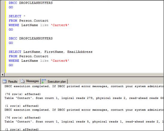
Confirming the improvement from a disk-statistics perspective, the logical reads drop significantly, from 279 to 5, as shown in figure 13.10.

Including additional columns in the nonclustered index to avoid the key lookup process makes it a covering index. While this is an excellent performance-tuning technique, the one downside is that the additional columns are included at all levels of the index (root, all intermediate levels, and the leaf level). In our query above, given that we're not using the additional columns as predicates, that is, where clause conditions, they're not required at any level of the index other than the leaf level to avoid the key lookup. In small indexes, this is not really an issue. However, for very large indexes, the additional space taken up by the additional columns at each index level not only increases the index size but makes the index seek process less efficient. The included columns feature, introduced in SQL Server 2005, enhances covering indexes in several ways.

Included columns

While they're a relatively simple and very effective performance-tuning mechanism, covering indexes are not without their limitations; there can be a maximum of 16 columns in a composite index with a maximum combined size of 900 bytes. Further, columns of certain data types, including n/varchar(max), n/varbinary(max), n/text, XML, and image cannot be specified as index key columns.

Recognizing the value of covering indexes, SQL Server 2005 and above circumvent the size and data type limitations through indexes with included columns. Such indexes allow additional columns to be added to the leaf level of nonclustered indexes. In doing so, the additional columns are not counted in the 16 column and 900 byte maximum, and additional data types are allowed for these columns (n/varchar(max), n/varbinary(max), and XML). Consider the following create index statement:

-- Include columns at the leaf level of the index
CREATE NONCLUSTERED INDEX ixContactLastName
ON Person.Contact (LastName)
INCLUDE (FirstName, EmailAddress)

Notice the additional INCLUDE clause at the end of the statement; this index will offer all the benefits of the previous covering index. Further, if appropriate, we could add columns with data types not supported in traditional indexes, and we wouldn't be restricted by the 16-column maximum.

When deciding whether to place a column in the index definition as a key column or as an included column, the determining factor is whether the column will be used as a predicate, that is, a search condition in the where clause of a query. If a column is added purely to avoid the key lookup because of inclusion in the select list, then it makes sense for it to be an included column. Alternatively, a column used for filtering/searching purposes should be included as a key column in the index definition.

Let's take our previous example of a surname search. If a common search condition was on the combination of surname and first name, then it would make sense for both columns to be included in the index as key columns for more efficient lookups when seeking through the intermediate index levels. If the email address column is used purely as return information, that is, in the query's select list, but not as a predicate (where clause condition), then it makes sense for it to be an included column. Such an index definition would look like this:

CREATE NONCLUSTERED INDEX ixContactLastName
ON Person.Contact (LastName, FirstName)
INCLUDE (EmailAddress)

In summary, included column indexes retain the power of covering indexes while minimizing the index size and therefore maximizing lookup efficiency.

Before closing our section on nonclustered index design, let's spend some time covering an important new indexing feature included in SQL Server 2008: filtered indexes.

Filtered indexes

Filtered indexes are one of my favorite new features in SQL Server 2008. Before we investigate their many advantages, consider the following table used to store customer details, including a country code:

CREATE TABLE [Person].[Customer](
   [CustomerID] [int] IDENTITY(1,1) PRIMARY KEY CLUSTERED

, [Title] [nvarchar](8) NULL
   , [FirstName] [nvarchar](100) NOT NULL
   , [LastName] [nvarchar](100) NOT NULL
   , [EmailAddress] [nvarchar](100) NULL
   , [CountryCode] char(2) NULL
)
GO

Let's imagine this table is part of a database used around the globe on a 24/7 basis. The Customer table is used predominantly by a follow-the-sun call center, where customer details are accessed by call center staff from the same country or region as the calling customers.

Creating a nonclustered index on this table similar to the one earlier in the chapter where we included FirstName, LastName, and EmailAddress will enable lookups on customer name to return the required details. If this was a very large table, the size of the corresponding nonclustered indexes would also be large. As we'll see later in the chapter, maintaining large indexes that are in use 24/7 presents some interesting challenges.

In our example here, a traditional (full table) index would be created similar to what we've already seen earlier in the chapter; columns would be defined as key or included index columns, ideally as part of a covering index. All is fine so far, but wouldn't it be good if we could have separate versions of the index for specific countries? That would enable, for example, the Australian version of the index to be rebuilt when it's midnight in Australia and few, if any, Australian users are being accessed. Such an index design would reduce the impact on sections of users that are unlikely to be accessed at the time of the index maintenance.

Consider the following two index-creation statements:

-- Create 2 filtered indexes on the Customer table
CREATE NONCLUSTERED INDEX ixCustomerAustralia
ON Person.Customer (LastName, FirstName)
INCLUDE (EmailAddress)
WHERE CountryCode = 'AU'
GO

CREATE NONCLUSTERED INDEX  ixCustomerUnitedKingdom
ON Person.Customer (LastName, FirstName)
INCLUDE (EmailAddress)
WHERE CountryCode = 'UK'
GO

The indexes we've created here are similar to ones from earlier in the chapter with one notable exception: they have a predicate (where clause filter) as part of their definition. When a search is performed using a matching predicate and index keys, the query optimizer will consider using the index, subject to the usual considerations. For example, the ixCustomerAustralia index could be used for a query that includes the CountryCode = 'AU' predicate such as this:

SELECT FirstName, LastName, EmailAddress
FROM Person.Customer
WHERE

LastName = 'Colledge'
   AND FirstName like 'Rod%'
   AND CountryCode = 'AU'

Such indexes, known as filtered indexes, enable a whole range of benefits. Let's cover the major ones:

• Segregated maintenance—As we've discussed, creating multiple smaller versions of a single larger index enables maintenance routines such as index rebuilds to be scheduled in isolation from other versions of the index that may be receiving heavy usage.

• Smaller, faster indexes—Filtering an index makes it smaller and therefore faster. Best of all, covered filtered indexes support optimized lookups for specialized purposes. Consider a very large product table with a ProductCategory column; filtered indexes could be created for product categories, which include the appropriate columns specific to that category. When combined with application logic, such indexes enable fast, optimized lookups for sections of data within a table.

• Creating unique indexes on nullable columns— Consider the Social Security number (SSN) column from earlier in the chapter; to support storing records for non-U.S. residents, we couldn't define the column as NOT NULL. This would mean that a percentage of the records would have a NULL SSN, but those that do have one should be unique. By creating a filtered unique nonclustered index, we can achieve both of these goals by defining the index with a WHERE SSN IS NOT NULL predicate.

• More accurate statistics—Unless created with the FULLSCAN option (covered later in the chapter), statistics work by sampling a subset of the index. In a filtered index, all of the sampled statistics are specific to the filter; therefore they are more accurate compared to an index that keeps statistics on all table data, some of which may never be used for index lookups.

• Lower storage costs—The ability to exclude unwanted data from indexes enables the size, and therefore storage costs, to be reduced.

Some of the advantages of filtered indexes could be achieved in earlier versions of SQL Server using indexed views. While similar, there are important differences and restrictions to be aware of when choosing one method over the other.

13.2.3. Indexed views

A traditional, nonindexed view provides a filter over one or more tables. Used for various purposes, views are an excellent mechanism for abstracting table join complexity and securing data. Indexed views, introduced in SQL Server 2000, materialize the results of the view. Think of an indexed view as another table with its own data, the difference being the data is sourced from one or more other tables. Indexed views are sometimes referred to as virtual tables.

To illustrate the power of indexed views, let's consider a modified example from SQL Server Books Online, where sales data is summarized by product and date. The original query, run against the base tables, is shown in listing 13.3.

Example 13.3. Sorted and grouped sales orders

-- Return orders grouped by date and product name
SELECT
    o.OrderDate
    , p.Name as productName
    , sum(UnitPrice * OrderQty * (1.00-UnitPriceDiscount)) as revenue
    , count_big(*) as salesQty
FROM Sales.SalesOrderDetail as od
    INNER JOIN Sales.SalesOrderHeader as o
      ON od.SalesOrderID = o.SalesOrderID
    INNER JOIN Production.Product as p
      ON od.ProductID = p.ProductID
WHERE o.OrderDate between '1 July 2001' and '31 July 2001'
GROUP BY o.OrderDate, p.Name
ORDER BY o.OrderDate, p.Name

What we're doing here is selecting the total sales (dollar total and count) for sales from July 2001, grouped by date and product. The I/O statistics for this query are as follows:

Table Worktable:

Scan count 0, logical reads 0, physical reads 0, read-ahead reads 0

Table SalesOrderDetail:

Scan count 184, logical reads 861, physical reads 1, read-ahead reads 8

Table SalesOrderHeader:

Scan count 1, logical reads 703, physical reads 1, read-ahead reads 699

Table Product:

Scan count 1, logical reads 5, physical reads 1, read-ahead reads 0

The AdventureWorks database is quite small, and as a result, the query completes in only a few seconds. On a much larger, real-world database, the query would take substantially longer, with a corresponding user impact. Consider the execution plan for this query, as shown in figure 13.11.

Figure 13.11. Query execution plan to return grouped, sorted sales data by date and product
 

The join, grouping, and sorting logic in this query are all contributing factors to its complexity and disk I/O usage. If this query was run once a day and after hours, then perhaps it wouldn't be much of a problem, but consider the user impact if this query was run by many users throughout the day.

Using indexed views, we can materialize the results of this query, as shown in listing 13.4.

Example 13.4. Creating an indexed view

-- Create an indexed view
CREATE VIEW Sales.OrdersView
WITH SCHEMABINDING
AS
    SELECT
        o.OrderDate
        , p.Name as productName
        , sum(UnitPrice * OrderQty * (1.00-UnitPriceDiscount)) as revenue
        , count_big(*) as salesQty
    FROM Sales.SalesOrderDetail as od
        INNER JOIN Sales.SalesOrderHeader as o
          ON od.SalesOrderID = o.SalesOrderID
        INNER JOIN Production.Product as p
          ON od.ProductID = p.ProductID
    GROUP BY o.OrderDate, p.Name
GO

--Create an index on the view
CREATE UNIQUE CLUSTERED INDEX ixv_productSales
    ON Sales.OrdersView (OrderDate, productName);
GO

Notice the WITH SCHEMABINDING used when creating the view. This essentially ties the view to the table definition, preventing structural table changes while the view exists. Further, creating the unique clustered index in the second half of the script is what materializes the results of the view to disk. Once materialized, the same query that we ran before can be run again, without needing to reference the indexed view.^[] The difference can be seen in the I/O statistics and dramatically simpler query execution plan, as shown in figure 13.12.

^[] This assumes the Enterprise edition is being used. Non-Enterprise editions require an explicit reference to the indexed view with the NOEXPAND hint.

Figure 13.12. Indexed views result in dramatically simpler execution plans and reduced resource usage. Compare this execution plan with the plan shown in figure 13.11.
 

Essentially, what we've done in creating the indexed view is store, or materialize, the results such that the base tables no longer need to be queried to return the results, thereby avoiding the (expensive) aggregation process to calculate revenue and sales volume. The I/O statistics for the query using the indexed view are as follows:

Table OrdersView:

Scan count 1, logical reads 5, physical reads 1, read-ahead reads 2

That's a total of 5 logical reads, compared to 1500-plus before the indexed view was created. You can imagine the accumulated positive performance impact of the indexed view if the query was run repeatedly throughout the day.

Once an indexed view is materialized with the unique clustered index, additional nonclustered indexes can be created on it; however, the same performance impact and index maintenance considerations apply as per a standard table.

Used correctly, indexed views are incredibly powerful, but there are several downsides and considerations. The primary one is the overhead in maintaining the view; that is, every time a record in one of the view's source tables is modified, the corresponding updates are required in the indexed view, including re-aggregating results if appropriate. The maintenance overhead for updates on the base tables may outweigh the read performance benefits; thus, indexed views are best used on tables with infrequent updates.

The other major consideration for creating indexed views is their constraints and base table requirements. Books Online contains a complete description of these constraints. The major ones are as follows:

• Schema binding on the base tables prevents any schema changes to the underlying tables while the indexed view exists.

• The index that materializes the view, that is, the initial clustered index, must be unique; hence, there must be a unique column, or combination of columns, in the view.

• The indexed view cannot include n/text or image columns.

The indexed view that we created in the previous example for sales data grouped by product and date was one of many possible implementations. A simpler example of an indexed view follows:

-- Create an indexed view
CREATE VIEW Person.AustralianCustomers
WITH SCHEMABINDING
AS
SELECT CustomerID, LastName, FirstName, EmailAddress
FROM Person.Customer
WHERE CountryCode = 'AU'
go

CREATE UNIQUE CLUSTERED INDEX ixv_AustralianCustomers
    ON Person.AustralianCustomers(CustomerID);
GO

If you recall our example from earlier in the chapter when we looked at filtered indexes, this essentially achieves the same thing. So which is the better method to use?

Indexed views vs. filtered indexes

We can use both filtered indexes and indexed views to achieve fast lookups for subsets of data within a table. The method chosen is based in part on the constraints and limitations of each method. We've covered some of the indexed view restrictions (schema binding, no n/text or image columns, and so forth). When it comes to filtered indexes, the major restriction is the fact that, like full table indexes, they can be defined on only a single table. In contrast, as you saw in our example with sales data, an indexed view can be created across many tables joined together.

Additional restrictions apply to the predicates for a filtered index. In our earlier example, we created filtered indexes with simple conditions such as where CountryCode = 'AU'. More complex predicates such as string comparisons using the LIKE operator are not permitted in filtered indexes, nor are computed columns.

Data type conversion is not permitted on the left-hand side of a filtered index predicate, for example, a table containing a varbinary(4) column named col1, with a filter predicate such as where col1 = 10. In this case, the filtered index would fail because col1 requires an implicit binary-to-integer conversion.^[]

^[] Changing the filtered index predicate to where col1 = convert(varbinary(4), 10) would be valid.

In summary, filtered indexes are best used against single tables with simple predicates where the row volume of the index is a small percentage of the total table row count. In contrast, indexed views are a powerful solution for multi-table join scenarios with aggregate calculations and more complex predicates on tables that are infrequently updated. Perhaps the major determining factor is the edition of SQL Server used. While indexed views can be created in any edition of SQL Server, they'll be automatically considered for use only in the Enterprise edition. In other editions, they need to be explicitly referenced with the NOEXPAND query hint.

With these index design points in mind, let's now look at processes and techniques for analyzing indexes to determine their usage and subsequent maintenance requirements.