
![]()
Grouping is primarily performed in SQL Server by using the GROUP BY clause in a SELECT query to determine in which groups rows should be put. Data is summarized by using the SUM function. The simplified syntax is as follows:
SELECT Column1, SUM(Column2)
FROM table_list
[WHERE search_conditions]
GROUP BY Column1
GROUP BY follows the optional WHERE clause and is most often used when aggregate functions are being utilized in the SELECT statement (aggregate functions are reviewed in more detail in Chapter 7).
5-1. Summarizing a Result Set
Problem
You need to know the total number of items in your warehouse.
Solution
Use the SUM function to add up the Quantity column values in your inventory table.
SELECT SUM(i.Quantity) AS Total
FROM   Production.ProductInventory i;
This query returns the following result set:
Total
------
335974
How It Works
The entire Production.ProductInventory table is scanned, and the Quantity column values are added up, and a sum is returned.
5-2. Creating Summary Groups
Problem
You need to summarize one column for every change in a second column. For example, you want to report the total amount due by an order date from the sales table. There are many orders per day, and you want to report only the total per day.
Solution
Group your detail data in the OrderDate column. Then apply the SUM function to the TotalDue column to generate a total due per date. This example uses the GROUP BY clause to summarize the total amount due by the order date from the Sales.SalesOrderHeader table:
SELECT OrderDate,
       SUM(TotalDue) AS TotalDueByOrderDate
FROM Sales.SalesOrderHeader
WHERE OrderDate >= '2005-07-01T00:00:00'
       AND OrderDate < '2005-08-01T00:00:00'
GROUP BY OrderDate;
This query returns the following (abridged) result set:
OrderDate               TotalDueByOrderDate
-----------------------	-------------------
2005-07-01 00:00:00.000	567020.9498
2005-07-02 00:00:00.000	15394.3298
2005-07-03 00:00:00.000	16588.4572
2005-07-30 00:00:00.000	15914.584
2005-07-31 00:00:00.000	16588.4572
How It Works
To determine the groups that rows should be put in, the GROUP BY clause is used in a SELECT query. Stepping through the first line of the query, the SELECT clause designates that the OrderDate should be returned, as well as the SUM total of values in the TotalDue column. SUM is an aggregate function. An aggregate function performs a calculation against a set of values (in this case TotalDue), returning a single value (the total of TotalDue by OrderDate):
SELECT OrderDate,
       SUM(TotalDue) AS TotalDueByOrderDate
Notice that a column alias for the SUM(TotalDue) aggregation is used. A column alias returns a different name for a calculated, aggregated, or regular column. In the next part of the query, the Sales.SalesOrderHeader table is referenced in the FROM clause.
FROM Sales.SalesOrderHeader
Next, the OrderDate is qualified to return rows for the month of July and the year 2005.
WHERE OrderDate >= '2005-07-01T00:00:00'
       AND OrderDate < '2005-08-01T00:00:00'
The result set is grouped by OrderDate (note that grouping can occur against one or more combined columns).
GROUP BY OrderDate;
If the GROUP BY clause were to have been left out of the query, using an aggregate function in the SELECT clause would have raised the following error:
Msg 8120, Level 16, State 1, Line 1
Column 'Sales.SalesOrderHeader.OrderDate' is invalid in the select list because
it is not contained in either an aggregate function or the GROUP BY clause.
This error is raised because any column that is not used in an aggregate function in the SELECT list must be listed in the GROUP BY clause.
5-3. Restricting a Result Set to Groups of Interest
Problem
You do not want to return all of the rows being returned by an aggregation; instead, you want only the rows where the aggregation itself is filtered. For example, you want to report on the reasons that the product was scrapped, but only for the reasons that have more than 50 occurrences.
Solution
Specify a HAVING clause, giving the conditions that the aggregated rows must meet in order to be returned.
This example queries two tables, Production.ScrapReason and Production.WorkOrder. The Production.ScrapReason table is a lookup table that contains manufacturing failure reasons, and the Production.WorkOrder table contains the manufacturing work orders that control which products are manufactured in the quantity and time period in order to meet inventory and sales needs. A report is needed that shows which of the “failure reasons” have occurred more than 50 times.
SELECT s.Name,
       COUNT(w.WorkOrderID) AS Cnt
FROM Production.ScrapReason s
       INNER JOIN Production.WorkOrder w
        ON s.ScrapReasonID = w.ScrapReasonID
GROUP BY s.Name
HAVING COUNT(*) > 50;
This query returns the following result set:
Name                               Cnt
------------------------------     ---
Gouge in metal                     54
Stress test failed                 52
Thermoform temperature too low     63
Trim length too long               52
Wheel misaligned                   51
How It Works
The HAVING clause of the SELECT statement allows you to specify a search condition on a query using GROUP BY and/or an aggregated value. The syntax is as follows:
SELECT select_list
FROM table_list
[ WHERE search_conditions ]
[ GROUP BY group_by_list ]
[ HAVING search_conditions ]
The HAVING clause is used to qualify the results after the GROUP BY has been applied. The WHERE clause, in contrast, is used to qualify the rows that are returned before the data is aggregated or grouped. HAVING qualifies the aggregated data after the data has been grouped or aggregated.
In this recipe, the SELECT clause requests a count of WorkOrderIDs by failure name:
SELECT s.Name,
       COUNT(w.WorkOrderID) AS Cnt
Two tables are joined by the ScrapReasonID column:
FROM Production.ScrapReason s
      INNER JOIN Production.WorkOrder w
        ON s.ScrapReasonID = w.ScrapReasonID
Because an aggregate function is used in the SELECT clause, the nonaggregated columns must appear in the GROUP BY clause:
GROUP BY s.Name
Lastly, using the HAVING query determines that, of the selected and grouped data, only those rows in the result set with a count of more than 50 will be returned:
HAVING COUNT(*)>50
5-4. Removing Duplicates from the Detailed Results
Problem
You need to know the quantity of unique values per date.
Solution
Add the DISTINCT clause to the COUNT function.
SELECT [RateChangeDate],
       COUNT([Rate]) AS [Count],
       COUNT(DISTINCT Rate) AS [DistinctCount]
FROM [HumanResources].[EmployeePayHistory]
WHERE RateChangeDate >= '2003-01-01T00:00:00.000'
       AND RateChangeDate < '2003-01-10T00:00:00.000'
GROUP BY RateChangeDate;
This query returns the following result set:
RateChangeDate              Count     DistinctCount
-----------------------     -----     -------------
2003-01-02 00:00:00.000     2          2
2003-01-03 00:00:00.000     3          2
2003-01-04 00:00:00.000     1          1
2003-01-05 00:00:00.000     3          3
2003-01-06 00:00:00.000     1          1
2003-01-07 00:00:00.000     2          2
2003-01-08 00:00:00.000     5          3
2003-01-09 00:00:00.000     2          2
How It Works
The previous query utilizes two COUNT functions; the second one also uses the DISTINCT clause. This forces the COUNT function to count only the distinct values in the specified column, in this case the Rate column.
5-5. Creating Summary Cubes
Problem
You need to return a data set with the detail data and with the data summarized on each combination of columns specified in the GROUP BY clause.
Solution
You need to include the CUBE argument after the GROUP BY clause. This example uses the CUBE argument to produce subtotal lines at the Shelf and LocationID levels, as well as a grand total.
SELECT i.Shelf,
       i.LocationID,
       SUM(i.Quantity) AS Total
FROM Production.ProductInventory i
GROUP BY CUBE(i.Shelf, i.LocationID);
This query produces several levels of totals, the first being by LocationID. The abridged result set is as follows:
Shelf     LocationID     Total
-----     ----------     -----
A          1             2727
C          1             13777
D          1             6551
…
J          1             5051
K          1             6751
L          1             7537
NULL       1             72899
Later in this result set, you will see totals by shelf and then across all shelves and locations.
Shelf     LocationID     Total
-----     ----------     ------
…
T          NULL          10634
U          NULL          18700
V          NULL          2635
W          NULL          2908
Y          NULL          437
NULL       NULL          335974
How It Works
By using the CUBE argument, the query groups by the specified columns, and it creates additional rows that provide totals for each combination of the columns specified in the GROUP BY clause.
CUBE uses a slightly different syntax from previous versions of SQL Server: CUBE is after the GROUP BY clause, instead of trailing the GROUP BY clause with a WITH CUBE. Notice also that the column lists are contained within parentheses.
![]() Note The GROUP BY WITH CUBE feature does not follow the ISO standard, and it will be removed in a future version of Microsoft SQL Server. You should avoid using this feature in any new development work, and you should modify any applications that currently use this feature to use the CUBE argument.
Note The GROUP BY WITH CUBE feature does not follow the ISO standard, and it will be removed in a future version of Microsoft SQL Server. You should avoid using this feature in any new development work, and you should modify any applications that currently use this feature to use the CUBE argument.
5-6. Creating Hierarchical Summaries
Problem
You need to return a data set with the detail data and with subtotals and grand total rows based upon the GROUP BY clause.
Solution
You need to include the ROLLUP argument after the GROUP BY clause. This example uses the ROLLUP argument to produce subtotal lines at the Shelf level, as well as a grand-total line.
SELECT i.Shelf,
       p.Name,
       SUM(i.Quantity) AS Total
FROM Production.ProductInventory i
       INNER JOIN Production.Product p
        ON i.ProductID = p.ProductID
GROUP BY ROLLUP(i.Shelf, p.Name);
This query returns the following abridged result set:
Shelf     Name                Total
-----     ---------------     ------
A         Adjustable Race     761
A         BB Ball Bearing     909
A         Bearing Ball        791
A         NULL                26833
…
B         Adjustable Race     324
B         BB Ball Bearing     443
B         Bearing Ball        318
B         NULL                12672
…
Y         HL Spindle/Axle     228
Y         LL Spindle/Axle     209
Y         NULL                437
NULL      NULL                335974
How It Works
The order you place the columns in the GROUP BY ROLLUP clause affects how data is aggregated. ROLLUP in this query aggregates the total quantity for each change in Shelf. Notice the row with shelf A and the NULL name; this holds the total quantity for shelf A. Also notice that the final row is the grand total of all product quantities. Whereas CUBE creates a result set that aggregates all combinations for the selected columns, ROLLUP generates the aggregates for a hierarchy of values.
GROUP BY ROLLUP (i.Shelf, p.Name)
ROLLUP aggregated a grand total and totals by shelf. Totals were not generated for the product name but would have been had CUBE been designated instead.
Just as CUBE does, ROLLUP uses slightly different syntax from previous versions of SQL Server. ROLLUP is after the GROUP BY, instead of trailing the GROUP BY clause with a WITH ROLLUP. Notice also that the column lists are contained within parentheses.
![]() Note The GROUP BY WITH ROLLUP feature does not follow the ISO standard, and it will be removed in a future version of Microsoft SQL Server. You should avoid using this feature in any new development work, and you should modify any applications that currently use this feature to use the ROLLUP argument.
Note The GROUP BY WITH ROLLUP feature does not follow the ISO standard, and it will be removed in a future version of Microsoft SQL Server. You should avoid using this feature in any new development work, and you should modify any applications that currently use this feature to use the ROLLUP argument.
5-7. Creating Custom Summaries
Problem
You need to have one result set with multiple custom aggregations.
Solution
You need to include the GROUPING SETS argument after the GROUP BY clause and include each of the custom aggregations that you want performed.
SQL Server gives you the ability to define your own grouping sets within a single query result set without having to resort to multiple UNION ALLs. GROUPING SETS also provides you with more control over what is aggregated, compared to the previously demonstrated CUBE and ROLLUP operations. This is performed by using the GROUPING SETS operator.
First, I demonstrate by defining an example business requirement for a query. Let’s assume I want a single result set to contain three different aggregate quantity summaries. Specifically, I would like to see quantity totals by shelf, quantity totals by shelf and product name, and then also quantity totals by location and name.
To achieve this in previous versions of SQL Server, you would have needed to use the UNION ALL operator.
SELECT NULL AS Shelf,
        i.LocationID,
        p.Name,
        SUM(i.Quantity) AS Total
FROM Production.ProductInventory i
        INNER JOIN Production.Product p
        ON i.ProductID = p.ProductID
WHERE Shelf IN ('A', 'C')
        AND Name IN ('Chain', 'Decal', 'Head Tube')
GROUP BY i.LocationID,
        p.Name
UNION ALL
SELECT i.Shelf,
        NULL,
        NULL,
        SUM(i.Quantity) AS Total
FROM Production.ProductInventory i
        INNER JOIN Production.Product p
        ON i.ProductID = p.ProductID
WHERE Shelf IN ('A', 'C')
        AND Name IN ('Chain', 'Decal', 'Head Tube')
GROUP BY i.Shelf
UNION ALL
SELECT i.Shelf,
        NULL,
        p.Name,
        SUM(i.Quantity) AS Total
FROM Production.ProductInventory i
        INNER JOIN Production.Product p
        ON i.ProductID = p.ProductID
WHERE Shelf IN ('A', 'C')
        AND Name IN ('Chain', 'Decal', 'Head Tube')
GROUP BY i.Shelf,
        p.Name;
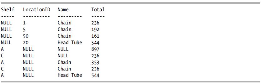
This query returns the following result set:
You can save yourself all that extra code by using the GROUPING SETS operator to define the various aggregations you would like to have returned in a single result set:
SELECT i.Shelf,
        i.LocationID,
        p.Name,
        SUM(i.Quantity) AS Total
FROM Production.ProductInventory i
        INNER JOIN Production.Product p
        ON i.ProductID = p.ProductID
WHERE Shelf IN ('A', 'C')
        AND Name IN ('Chain', 'Decal', 'Head Tube')
GROUP BY GROUPING SETS((i.Shelf),
        (i.Shelf, p.Name),
        (i.LocationID, p.Name));
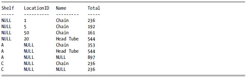
This returns the same result set as the previous query (only ordered a little differently):
How It Works
The new GROUPING SETS operator allows you to define varying aggregate groups in a single query while avoiding having multiple queries attached together using the UNION ALL operator. The core of this recipe’s example is the following two lines of code:
GROUP BY GROUPING SETS
((i.Shelf), (i.Shelf, p.Name), (i.LocationID, p.Name))
Notice that unlike a regular aggregated query, the GROUP BY clause is not followed by a list of columns. Instead, it is followed by GROUPING SETS. GROUPING SETS is then followed by parentheses and the groupings of column names, each also encapsulated in parentheses.
5-8. Identifying Rows Generated by the GROUP BY Arguments
Problem
You need to differentiate between the rows that actually have stored NULL data and the rows generated by the GROUP BY arguments that have a NULL generated for that column.
Solution
You need to utilize the GROUPING function in your query.
The following query uses a CASE statement to evaluate whether each row is a total by shelf, total by location, grand total, or regular noncubed row:
SELECT i.Shelf,
        i.LocationID,
        CASE WHEN GROUPING(i.Shelf) = 0
                  AND GROUPING(i.LocationID) = 1 THEN 'Shelf Total'
             WHEN GROUPING(i.Shelf) = 1
                  AND GROUPING(i.LocationID) = 0 THEN 'Location Total'
             WHEN GROUPING(i.Shelf) = 1
                  AND GROUPING(i.LocationID) = 1 THEN 'Grand Total'
             ELSE 'Regular Row'
        END AS RowType,
        SUM(i.Quantity) AS Total
FROM     Production.ProductInventory i
WHERE    LocationID = 2
GROUP BY CUBE(i.Shelf, i.LocationID);
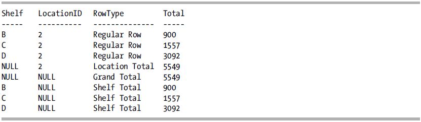
This query returns the following result set:
How It Works
You may have noticed that the rows grouped in the previous recipes have NULL values in the columns that aren’t participating in the aggregate totals. For example, when shelf C is totaled up in Recipe 5-6, the location and product name columns are NULL:
C NULL NULL 236
The NULL values are acceptable if your data doesn’t explicitly contain NULLs; however, what if it does? How can you differentiate “stored” NULLs from those generated in the rollups, cubes, and grouping sets? To address this issue, you can use the GROUPING function.
The GROUPING function allows you to differentiate and act upon those rows that are generated automatically for aggregates using CUBE, ROLLUP, and GROUPING SETS. In this example, the SELECT statement starts off normally, with the Shelf and Location columns:
SELECT i.Shelf, i.LocationID,
Following this is a CASE statement that would evaluate the combinations of return values for the GROUPING statement.
![]() Tip For more on CASE, see Chapter 2.
Tip For more on CASE, see Chapter 2.
When GROUPING returns a 1 value (true), it means the column NULL is not an actual data value but is a result of the aggregate operation, standing in for the value all. So, for example, if the shelf value is not NULL and the location ID is NULL because of the CUBE aggregation process and not the data itself, the string Shelf Total is returned:
CASE WHEN GROUPING(i.Shelf) = 0
          AND GROUPING(i.LocationID) = 1 THEN 'Shelf Total'
This continues with similar logic, only this time if the shelf value is NULL because of the CUBE aggregation process but the location is not null, a location total is provided:
WHEN GROUPING(i.Shelf) = 1
     AND GROUPING(i.LocationID) = 0 THEN 'Location Total'
The last WHEN defines when both shelf and location are NULL because of the CUBE aggregation process, which means the row contains the grand total for the result set:
WHEN GROUPING(i.Shelf) = 1
     AND GROUPING(i.LocationID) = 1 THEN 'Grand Total'
GROUPING returns only a 1 or a 0; however, in SQL Server, you also have the option of using GROUPING_ID to compute grouping at a finer grain, as I demonstrate in the next recipe.
5-9. Identifying Summary Levels
Problem
You need to identify which columns are being considered in the grouping rows added to the result set.
Solution
You need to utilize the GROUPING_ID function in your query.
The following query uses the GROUPING_ID function to return those columns used in the grouping of that particular row:
SELECT i.Shelf,
        i.LocationID,
        i.Bin,
        CASE GROUPING_ID(i.Shelf, i.LocationID, i.Bin)
          WHEN 1 THEN 'Shelf/Location Total'
          WHEN 2 THEN 'Shelf/Bin Total'
          WHEN 3 THEN 'Shelf Total'
          WHEN 4 THEN 'Location/Bin Total'
          WHEN 5 THEN 'Location Total'
          WHEN 6 THEN 'Bin Total'
          WHEN 7 THEN 'Grand Total'
          ELSE 'Regular Row'
        END AS GroupingType,
        SUM(i.Quantity) AS Total
FROM     Production.ProductInventory i
WHERE    i.LocationID IN (3)
         AND i.Bin IN (1, 2)
GROUP BY CUBE(i.Shelf, i.LocationID, i.Bin)
ORDER BY i.Shelf,
         i.LocationID,
         i.Bin;
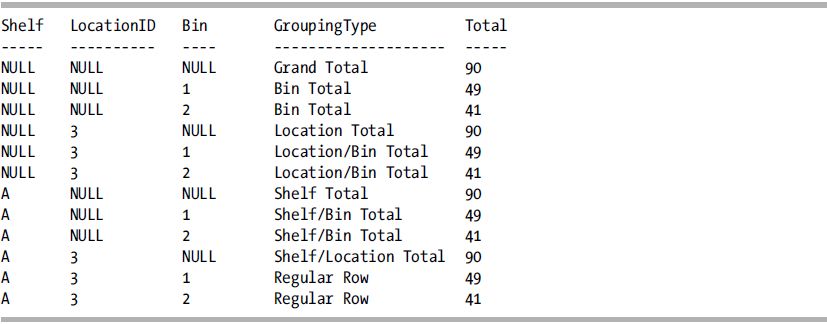
The result set returned from this query has descriptions of the various aggregations CUBE resulted in.
How It Works
![]() Note This recipe assumes an understanding of the binary/base-2 number system.
Note This recipe assumes an understanding of the binary/base-2 number system.
Identifying which rows belong to which type of aggregate becomes progressively more difficult for each new column you add to the GROUP BY clause and for each unique data value that can be grouped and aggregated. For example, this query shows the quantity of products in location 3 within bins 1 and 2:
SELECT i.Shelf,
       i.LocationID,
       i.Bin,
       i.Quantity
FROM   Production.ProductInventory i
WHERE  i.LocationID IN (3)
       AND i.Bin IN (1, 2);
This query returns only two rows:
Shelf     LocationID     Bin     Quantity
-----     ----------     ---     --------
A         3              2       41
A         3              1       49
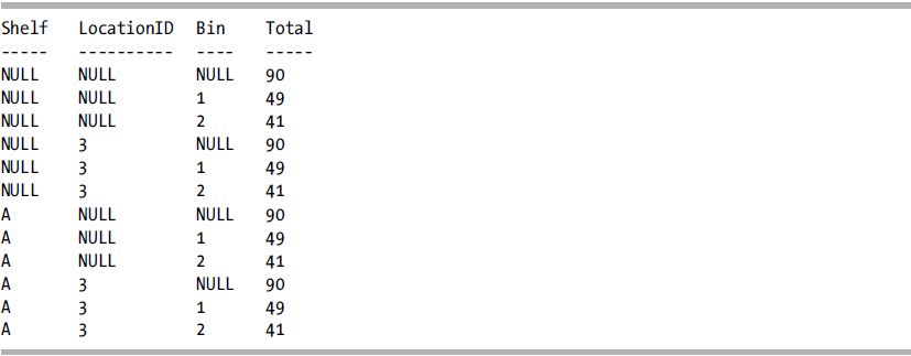
Now what if we needed to report aggregations based on the various combinations of Shelf, Location, and Bin? We could use CUBE to give summaries of all these potential combinations:
SELECT   i.Shelf,
         i.LocationID,
         i.Bin,
         SUM(i.Quantity) AS Total
FROM     Production.ProductInventory i
WHERE    i.LocationID IN (3)
         AND i.Bin IN (1, 2)
GROUP BY CUBE(i.Shelf, i.LocationID, i.Bin)
ORDER BY i.Shelf,
         i.LocationID,
         i.Bin;
Although the query returns the various aggregations expected from CUBE, the results are difficult to decipher.
This is where GROUPING_ID comes in handy. Using this function, we can determine the level of grouping for the row. This function is more complicated than GROUPING, however, because GROUPING_ID takes one or more columns as its input and then returns the integer equivalent of the base-2 (binary) number calculation on the columns.
In analyzing the query in the solution, GROUPING_ID takes a column list and returns the integer value of the base-2 binary column list calculation. Stepping through this, the query started off with the list of the three nonaggregated columns to be returned in the result set:
SELECT i.Shelf,
       i.LocationID,
       i.Bin,
Next, a CASE statement evaluates the return value of GROUPING_ID for the list of the three columns:
CASE GROUPING_ID(i.Shelf, i.LocationID, i.Bin)
To illustrate the base-2 conversion to integer concept, let’s focus on a single row, namely, the row that shows the grand total for shelf A generated automatically by CUBE:
Shelf     LocationID     Bin     Total
-----     ----------     ----    -----
NULL      NULL           NULL    90
Now envision another row beneath it that shows the bit values being enabled or disabled based on whether the column is a grouping column. Both Location and Bin from GROUPING_ID’s perspective have a bit value of 1 because neither of them is a grouping column for this specific row. For this row, Shelf is the grouping column. Let’s also add a third row that shows the integer value beneath the flipped bits:
Shelf     LocationID     Bin
-----     ----------     ----
A         NULL           NULL
0         1              1
4         2              1
Because only the location and bin have enabled bits, we add 1 and 2 to get a summarized value of 3, which is the value returned for this row by GROUPING_ID. So, the various grouping combinations are calculated from binary to integer. In the CASE statement that follows, 3 translates to a shelf total.
Because there are three columns, the various potential aggregations are represented in the following WHENs/THENs:
CASE GROUPING_ID(i.Shelf,i.LocationID, i.Bin)
     WHEN 1 THEN 'Shelf/Location Total'
     WHEN 2 THEN 'Shelf/Bin Total'
     WHEN 3 THEN 'Shelf Total'
     WHEN 4 THEN 'Location/Bin Total'
     WHEN 5 THEN 'Location Total'
     WHEN 6 THEN 'Bin Total'
     WHEN 7 THEN 'Grand Total'
ELSE 'Regular Row'
END,
Each potential combination of aggregations is handled in the CASE statement. The rest of the query involves using an aggregate function on quantity and then using CUBE to find the various aggregation combinations for the shelf, location, and bin:
       SUM(i.Quantity) AS Total
 FROM  Production.ProductInventory i
 WHERE i.LocationID IN (3)
  AND  i.Bin IN (1, 2)
 GROUP BY CUBE (i.Shelf, i.LocationID, i.Bin)
 ORDER BY i.Shelf, i.LocationID, i.Bin;